Nelson-Siegel-Svennson model for interest rates

A common approach that can be used to fit the interest rates for different maturities given a set of key-rates is linear interpolation. However a more flexible approach, often used by central banks, is to calibrate the parameters of a model and then to use it to recover the interest rate for any time to maturity. In Equation 1 we present a modified version of the original Nelson-Siegel model, called Nelson-Siegel-Svennson model, in which are introduced two additional parameters, \(\beta_3\) and \(\tau_2\), in order to have more flexibility. Thus the parameter vector is \(\theta = (\beta_0,\beta_1, \beta_2, \beta_3, \tau_1, \tau_2)\). \[ \hat{h}(0,T) = \beta_0 + \beta_1 f^1(T, \tau_1) + \beta_2 f^2(T, \tau_1) + \beta_3 f^2(T, \tau_2) \tag{1}\] where: \[ f^1(T,\tau_1) = \frac{1 - e^{-\frac{T}{\tau_1}}}{\frac{T}{\tau_1}} \tag{2}\] and \[ f^2(T,\tau) = \frac{1 - e^{-\frac{T}{\tau}}}{\frac{T}{\tau}} - e^{-\frac{T}{\tau}} \tag{3}\]

Under the Nelson-Siegel model, the first two parameters, namely \(\beta_0\) and \(\beta_1\), can be interpreted as follows:

• \(\beta_0\) as the long term interest rate;
• \(\beta_0 + \beta_1\) as instantaneous short term interest rate.

To ensure that these constraints are satisfied in the optimization problem, namely to satisfy: \[ \beta_0 + \beta_1 = h(0,T) \tag{4}\] we can reparametrize the first parameter \(\beta_0\) to be \(\beta_0(\beta_1) = h(0,T) - \beta_1\) and thus satisfying Equation 4.

Then, given this reparametrization one can proceed by minimizing the MSE between the realized and fitted yield curve, i.e.  \[ \underset{\tiny \beta_0(\beta_1), \beta_1, \beta_2, \beta_3, \tau_1, \tau_2}{\text{argmin}}\biggl\{ \sum_{i = a}^{i = b} \bigl[ h(0,T_i) - \hat{h}(0,T_i) \bigl]^2 \biggl\} \tag{5}\] Subject to the constraint: where \((T_a, ....T_b)\) is a set of discrete maturities.

#' Nelson Siegel function 
#' @param tau vector of times to maturity 
#' @param params vector of parameters with order (beta0, beta1, beta2, beta3, tau1, tau2)
#' @return vector of yields
nelson_siegel <- function(tau, params){
  # Parameters 
  beta0 = params[1]
  beta1 = params[2]
  beta2 = params[3]
  beta3 = params[4]
  tau1 = params[5]
  tau2 = params[6]
  # Auxiliary function 1
  f1 <- function(tau, theta){
    exp(-tau/theta)
  }
  # Auxiliary function 2
  f2 <- function(tau, theta){ 
    (1 - f1(tau, theta))/(tau/theta)
  }
  # Auxiliary function 3
  f3 <- function(tau, theta){ 
    f2(tau, theta) - f1(tau, theta)
  }
  # Fit function  
  beta0 + beta1 * f2(tau, tau1) + beta2 * f3(tau, tau1) + beta3 * f3(tau, tau2)
}

1 Example: estimation

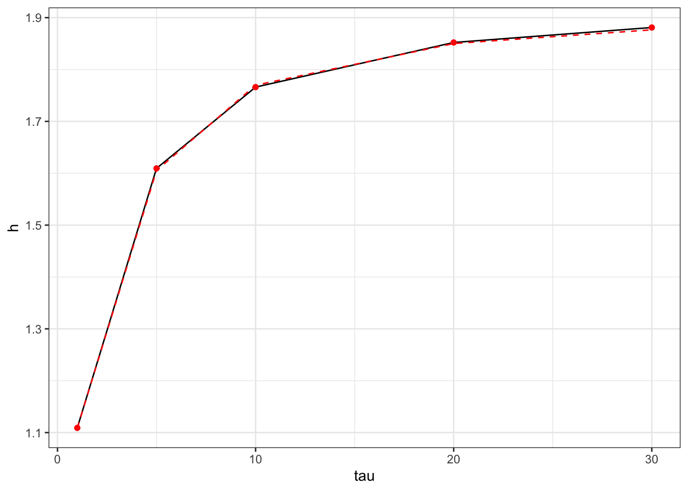
Let’s consider a yield curve equal to \(h(0,T) = (1.1091 \%, 1.6094 \%, 1.7661 \%, 1.8521 \%, 1.881 \%)\) with maturities \(T = (1, 5, 10, 20, 30)\) years.

In order to find the optimal parameters, it is necessary to solve a minimization problem starting from a set of 5 parameters, in general arbitrary or randomly generated. In this case, the following algorithm was implemented:

1. Fix \(\beta_1\) both equal to \(\frac{h(0,t_1)}{2}\), in such a way the initial parameters respect the constraint in Equation 4.
2. Recover \(\beta_0\) as function of \(\beta_1\), i.e. \(\beta_0(\beta_1) = h(0,T) - \beta_1\).
3. Perform a standard uncontraint minimization problem in Equation 5 where the constraints are satisfied by the reparametrization.

fit_nelson_siegel <- function(h = NULL, tau = NULL, init_params = NULL){
  
  if (is.null(init_params)) {
    init_params <- rep(0.1, 6)
  }
  # Set the constraint for beta0 and beta1, i.e.
  # beta0 + beta1 = h(0, T) thus
  # beta0 = h(0, T) - beta1 
  # (beta1, beta2, beta3, tau1, tau2)
  init_params <- c(h[1]/2, init_params[3:6])
  
  loss_function <- function(params){
    # Compute beta0 from contraint 
    beta0 = h[1] - params[1] 
    # Full parameter vector 
    h_hat <- nelson_siegel(tau, c(beta0, params))
    sum((h - h_hat)^2)
  }
  # Minimize MSE 
  opt <- optim(init_params, loss_function)
  # Extract optimal parameters 
  opt_params <- c(beta0 = h[1] - opt$par[1], 
                  beta1 = opt$par[1], 
                  beta2 = opt$par[2],
                  beta3 = opt$par[3],
                  tau1  = opt$par[4], 
                  tau2  = opt$par[5])
  # Fitted yield curves 
  h_hat <- nelson_siegel(tau, opt_params)
  # MSE 
  mse <- sd(h_hat - h)

  list( 
    h = h,
    h_hat = h_hat, 
    mse = mse,
    init_params  = init_params,
    optim_params = opt_params
  )
}

# euribor 2022-11-16
h <- c(1.1091, 1.6094, 1.7661, 1.8521, 1.881)
# times to maturities in years
tau <- c(1, 5, 10, 20, 30)
# calibrate parameters 
fit <- fit_nelson_siegel(h = h, tau = tau, init_params = NULL)
# fitted yields under Nelson-Siegel 
h_pred <- nelson_siegel(tau, fit$optim_params)

library(ggplot2)
ggplot()+
  geom_line(aes(tau, h))+
  geom_point(aes(tau, h), color = "red")+
  geom_line(aes(tau, h_pred), linetype="dashed", color="red")+
  theme_bw()

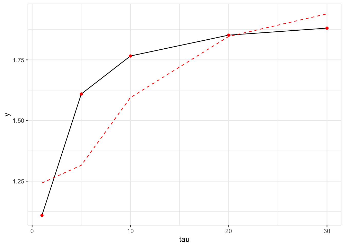
Note that under the reparametrization in \(\beta_0(\beta_1) = h(0,T) - \beta_1\), rescaling the rates/yield in the interval \([0,1]\) and then scaling back could cause problems in fitting resulting in an higher mse.

# euribor 2022-11-16
h <- c(1.1091, 1.6094, 1.7661, 1.8521, 1.881)
# times to maturities in years
tau <- c(1, 5, 10, 20, 30)

# calibrate parameters 
fit2 <- fit_nelson_siegel(h = h/100, tau = tau, init_params = NULL)
# fitted yields under Nelson-Siegel 
h_pred2 <- nelson_siegel(tau, fit2$optim_params)*100

library(ggplot2)
ggplot()+
  geom_line(aes(tau, h))+
  geom_point(aes(tau, h), color = "red")+
  geom_line(aes(tau, h_pred2), linetype="dashed", color="red")+
  theme_bw()

In this case, when we fit directly on the percentage yield we get an MSE of 5^{-5}, while when we scale 0.01225.