Bitcoin is volatile? – CryptoverseR

1 Introduction

Bitcoin, a digital currency known for its volatility, presents unique opportunities and challenges for those who rely on it as a medium of wealth and transactions. One interesting scenario to explore is the financial implications of converting a regular salary into Bitcoin at the start of each month and then converting smaller amounts back to fiat currency as needed for expenses throughout the month.

This study simulates such a setup, focusing on how Bitcoin’s price fluctuations affect purchasing power, spending, and financial planning. Understanding this relationship offers insights into Bitcoin’s utility as a practical currency and how fluctuations can impact daily living costs for those who choose to hold their income in Bitcoin.

Setup

library(tidyverse)
# ==========================================
# random seed for simulation of expenses
seed <- 1 
# Annual salary
yearly_salary <- 30000 
# Monthly salary 
monthly_salary <- yearly_salary/12
# Annual expenses 
yearly_expenses <- 21000 
# Monthly expenses 
monthly_expenses <- yearly_expenses/12
# Number of expenses. 
# Each occurs in a different day,
n_expenses <- 20 
# Amount for a single expense 
single_expense <- monthly_expenses/n_expenses
# Start date of the backtesting
start_conversion <- as.Date("2020-01-01")

To analyze this scenario, we establish a few key parameters based on typical income and spending patterns. This model assumes a fixed annual salary, a monthly breakdown of expenses, and a set number of transactions throughout the month to cover daily needs. The following parameters have been initialized:

Annual salary: set to represent a moderate income level for this analysis.
Monthly salary and expenses: calculated by dividing annual amounts by 12, representing a standard monthly budgeting approach.
Number of expenses: chosen to simulate the pattern of frequent, smaller expenditures typical of daily spending.

By using these simplified financial parameters, we create a consistent basis for analyzing the effects of Bitcoin’s price volatility on month-to-month financial stability.

Dataset

# Dataset of prices (15m data)
BTCUSDT <- read_csv("BTCUSDT-spot-15m.csv")

data <- mutate(BTCUSDT, 
               Day = as.Date(date), 
               Month = lubridate::month(date), 
               Year = lubridate::year(date))
data <- select(data, Year, Month, Day, date, close) 

# End date of the backtesting. Occur at the beginning of the month.
end_conversion <- as.Date(max(data$date)) - lubridate::day(max(data$date))
# conversion of monthly salary happen every 1 month
index <- seq.Date(start_conversion, end_conversion, by = "1 month")

Variable	Value
BTC data:	From 2020-01-01 to 2024-03-31
Yearly salary:	30000 USD
Yearly expenses:	21000 USD
$\frac{\text{expenses}}{\text{salary}}$:	70 %
Number monthly expenses:	20
Single expense:	87.5 USD

In practice, in this setup we earn 30000 USD each year, but we spent 21000 that is the 70 % of our annual income. Each month we convert our BTC 20 times for a mean value of 87.5 USD. Hence, our annual savings, the 30 % of the annual salary, will be stored in BTC instead of USD.

2 Bitcoin as an everyday currency?

This section simulates a typical month’s worth of expenses, which are randomly distributed across different days. Each expense represents a conversion from Bitcoin to fiat currency, dependent on the prevailing Bitcoin price at the time of conversion. This randomness in spending provides a realistic scenario where day-to-day needs dictate spending, rather than being able to plan conversions for optimal market timing. In this setup:

Each expense is a fixed fraction of the total monthly expenses.
Expenses occur on randomly selected days, aligning with the unpredictable nature of everyday spending.

The randomness of expenses introduces a layer of unpredictability, allowing us to observe how Bitcoin’s volatility affects cash flow stability and the ability to meet daily financial obligations. Hence, we simulate the conversion and expenses starting from 2020-01-01 up to 2024-03-31.

Expenses simulation

set.seed(seed)
result <- list()
all_result <- list()
for(i in 1:length(index)){
  # Number of the month (1-12)
  idx_month <- lubridate::month(index[i])
  # Number of year
  idx_year <- lubridate::year(index[i])
  # Conversion of salary occurs randomly on 1st of the month 
  payment_data <- dplyr::filter(data, Day == index[i]) 
  # Conversion price 
  btc_conversion_price <- payment_data$close[sample(nrow(payment_data), 1)]
  # Conversion amount 
  btc_conversion_amount <- monthly_salary/btc_conversion_price
  # Dataset for the month 
  month_data <- dplyr::filter(data, Month == idx_month & Year == idx_year) 
  # Add random conversion price 
  month_data$btc_price <- btc_conversion_price
  # Add random conversion amount 
  month_data$btc_amount <- btc_conversion_amount
  # Initialize expenses variables 
  month_data$expenses <- 0 
  month_data$btc_expenses <- 0 
  month_data$expenses_cost <- 0
  # Sample random expenses 
  idx_expenses <- sample(nrow(month_data), n_expenses, replace = FALSE)
  # Expenses amount in BTC
  btc_expenses <- single_expense/month_data[idx_expenses,]$close
  month_data$btc_expenses[idx_expenses] <- btc_expenses
  # Sampled expenses costs in USD
  month_data$expenses_cost[idx_expenses] <- btc_expenses*btc_conversion_price
  # Add expenses amount in USD
  month_data$expenses[idx_expenses] <- single_expense
  # Save data 
  all_result[[i]] <- month_data
  # Save monthly data 
  result[[i]] <- dplyr::tibble(
    date = index[i], 
    salary = monthly_salary, 
    btc_amount = btc_conversion_amount, 
    btc_price = btc_conversion_price,
    btc_vol = sd(month_data[idx_expenses,]$close),
    usd_monthly_expenses = monthly_expenses, 
    btc_monthly_expenses = sum(month_data$btc_expenses[idx_expenses]),
    btc_monthly_cost = sum(month_data$expenses_cost[idx_expenses]))
}
result <- dplyr::bind_rows(result) 
result <- dplyr::mutate(result, 
                        net_expenses = usd_monthly_expenses - btc_monthly_cost, 
                        usd_savings = salary - usd_monthly_expenses,
                        btc_savings = btc_amount - btc_monthly_expenses)
# Cumulated expenses in USD 
result$cum_usd_expenses <- cumsum(result$usd_monthly_expenses)
# Cumulated random expenses in BTC 
result$cum_btc_expenses <- cumsum(result$btc_monthly_cost)
# Cumulated savings in USD 
result$cum_usd_savings_usd <- cumsum(result$usd_savings)
# Cumulated random savings in BTC -> USD
result$cum_btc_savings_usd <- cumsum(result$btc_savings)*result$btc_price
# Cumulated savings in USD -> BTC
result$cum_usd_savings_btc <- cumsum(result$usd_savings)/result$btc_price
# Cumulated random savings in BTC
result$cum_btc_savings_btc <- cumsum(result$btc_savings)

We distinguish between two situations:

A positive expense occurs when the mean price at which we have converted the BTC during the month is above the buy price for that month and hence realize a gain.
A negative expense occurs when the mean price at which we have converted the BTC during the month is below the buy price price and hence realize a loss.

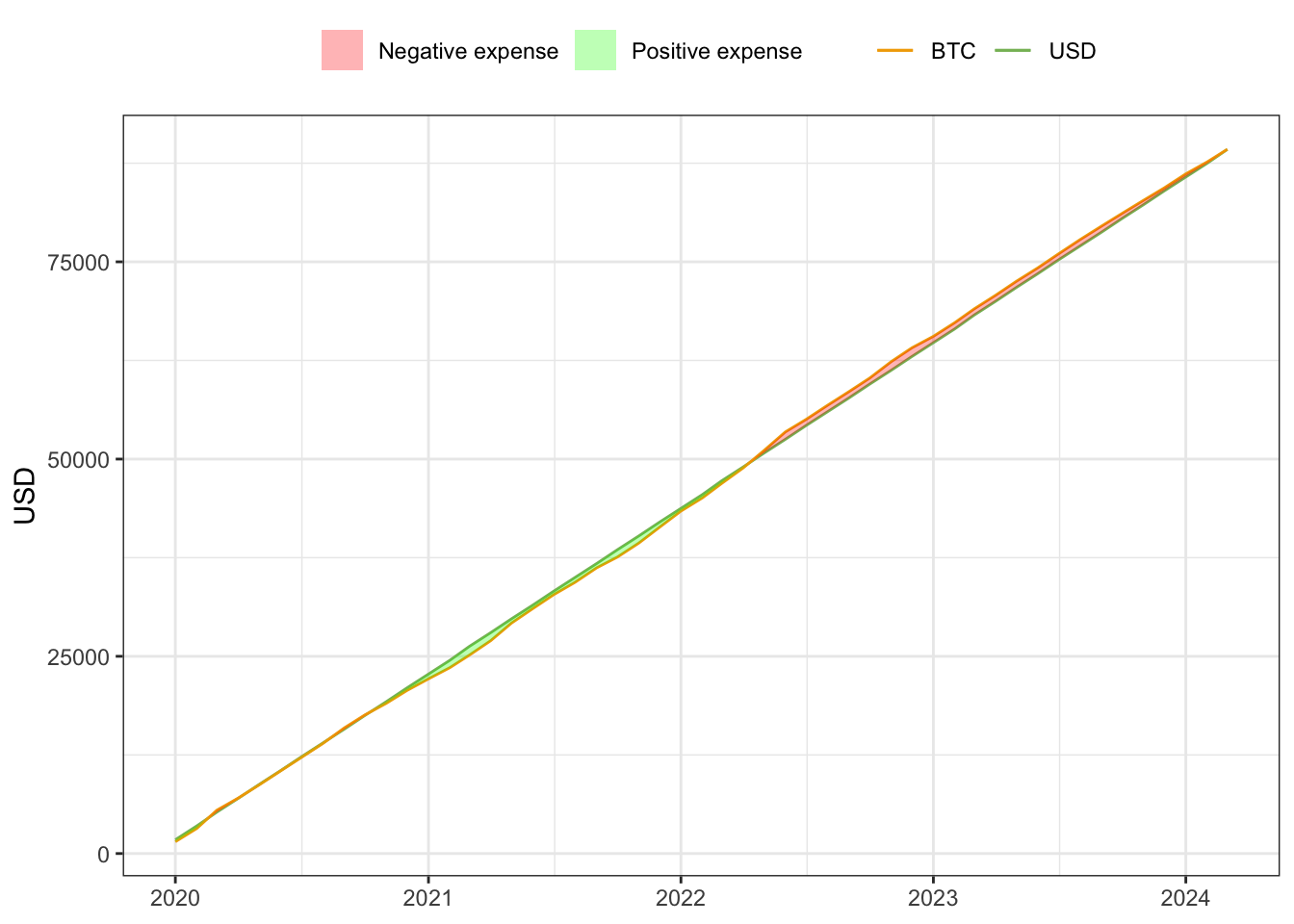
In Figure 1 we show the cumulated expenses in the two cases:

USD: where we we use only dollars for expenses.
BTC: where we use dollars for expenses, but we convert the salary in BTC and then BTC to USD only when an expense occurs.

Show the code

mycol <- list(btc = "#F2A900", usd = "#85bb65")
ggplot(result) +
  geom_line(aes(date, cum_usd_expenses, color = "usd")) +
  geom_line(aes(date, cum_btc_expenses, color = "btc")) +
  geom_ribbon(aes(x = date, xmin= min(date), xmax = max(date), 
                  ymin = cum_usd_expenses, ymax = cum_btc_expenses, 
                  fill = cum_usd_expenses > cum_btc_expenses)) +
  scale_color_manual(values = c(btc = mycol$btc, usd = mycol$usd), 
                     labels = c(btc = "BTC", usd = "USD")) + 
  scale_fill_manual(values = c(`TRUE` = "green", `FALSE` = "red"), 
                    labels = c(`TRUE` = "Positive expense", `FALSE` = "Negative expense")) +
  theme_bw() +
  theme(legend.position = "top") +
  labs(colour = NULL, fill = NULL, x = NULL, y = "USD")

Figure 1: Cumulated expenses in the two cases.

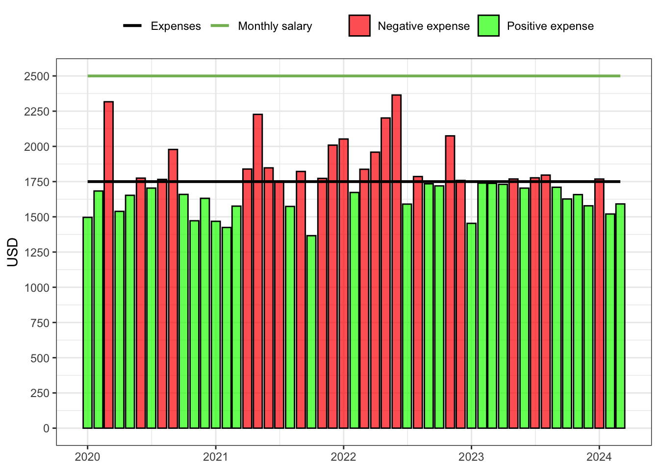
In Figure 2 we show the same situation but on a monthly basis. Moreover, even in months where we spend more, the difference with respect to the USD spending is not evident.

Show the code

y_breaks <- c(seq(0, monthly_salary, by = 250))
y_labels <- format(round(y_breaks), digits = 1)

ggplot(result) +
  geom_bar(aes(date, btc_monthly_cost, fill = btc_monthly_cost < usd_monthly_expenses), 
           stat = "identity", color = "black", alpha = 0.7)+
  geom_line(aes(date, monthly_salary, color = "salary"), size = 1)+
  geom_line(aes(date, usd_monthly_expenses, color = "expense"), size = 1)+
  scale_fill_manual(values = c(`TRUE` = "green", `FALSE` = "red"),
                    labels = c(`TRUE` = "Positive expense", `FALSE` = "Negative expense"))+
  scale_color_manual(values = c(expense = "black", salary = mycol$usd), 
                     labels = c(expense = "Expenses", salary = "Monthly salary"))+ 
  scale_y_continuous(breaks = y_breaks, labels = y_labels)+
  theme_bw()+
  theme(legend.position = "top")+
  labs(fill = NULL, color = NULL, y = "USD", x = NULL)

Figure 2: Monthly expenses in the two cases.

In fact, in Table 1, we compute the precise values of the cumulated expenses in both cases we can see that such difference is very small.

Show the code

last_cum_usd_expenses <- result$cum_usd_expenses[nrow(result)]
last_cum_btc_expenses <- result$cum_btc_expenses[nrow(result)]
tibble(
  btc_expenses = result$cum_usd_expenses[nrow(result)],
  usd_expenses = result$cum_btc_expenses[nrow(result)],
  tot_difference = abs(btc_expenses - usd_expenses),
  monthly_difference = tot_difference/nrow(result)
) %>%
  rename(`BTC Expenses` = "btc_expenses", `USD Expenses` = "usd_expenses", 
         `Global Difference` = "tot_difference", `Monthly Difference` = "monthly_difference") %>%
  mutate_all(function(x) paste0(round(x), " \\$")) %>%
  knitr::kable(escape = FALSE, booktabs=TRUE) %>%
  kableExtra::kable_classic_2()

Table 1: Cumulated expenses at the end of the period considered.

BTC Expenses	USD Expenses	Global Difference	Monthly Difference
89250 \$	89064 \$	186 \$	4 \$

2.1 Savings in BTC or in USD?

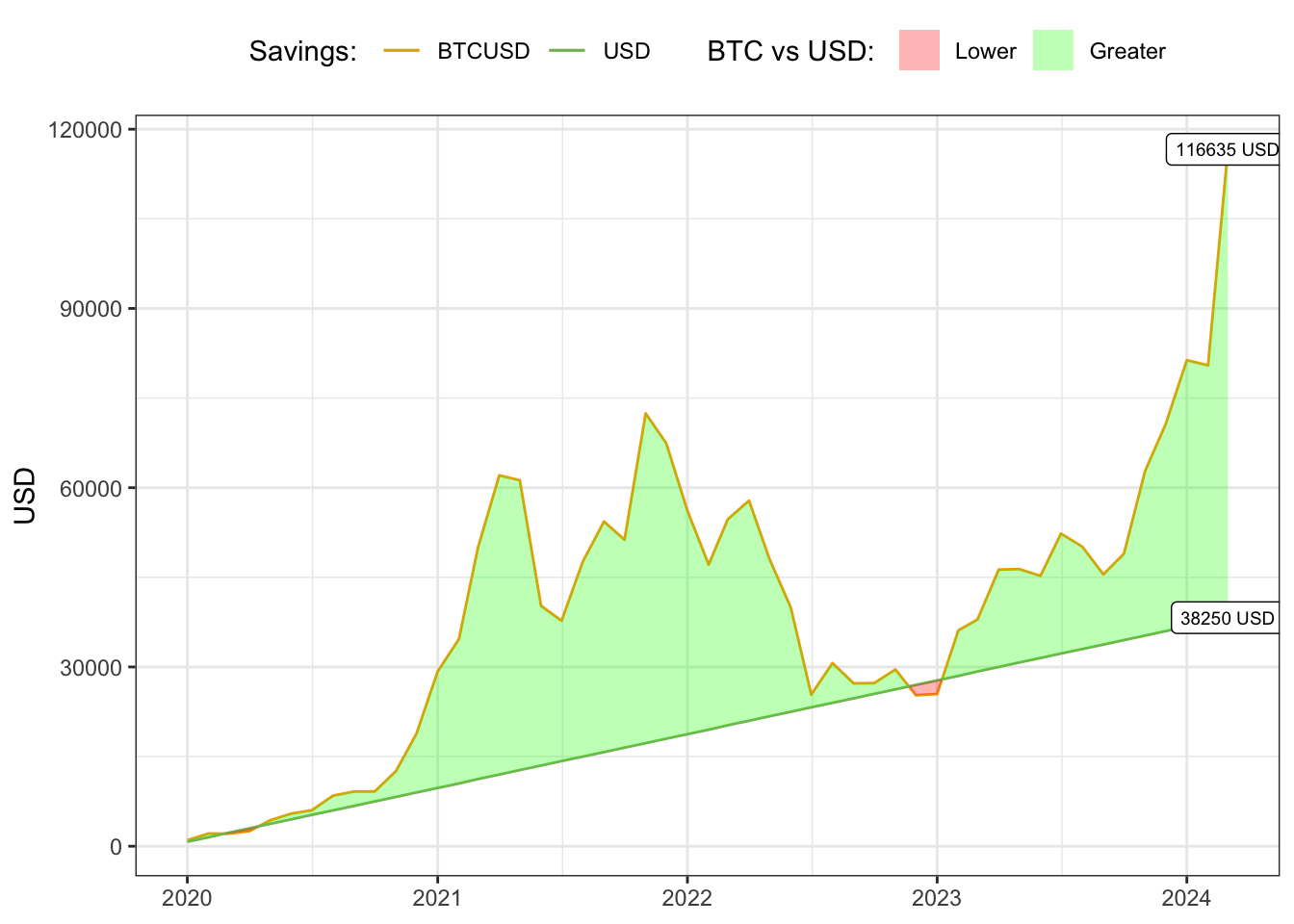
Here we compare the value of the savings in both cases expressed in USD.

Show the code

last_cum_usd_savings <- result$cum_usd_savings_usd[nrow(result)]
last_cum_btc_savings <- result$cum_btc_savings_usd[nrow(result)]

result %>%
  ggplot() +
  geom_line(aes(date, cum_btc_savings_usd,  color = "btc")) +
  geom_line(aes(date, cum_usd_savings_usd, color = "usd")) +
  scale_color_manual(values = c(btc = mycol$btc, usd = mycol$usd), 
                     labels = c(btc = "BTCUSD", usd = "USD"))+ 
  scale_fill_manual(values = c(`TRUE` = "green", `FALSE` = "red"),
                    labels = c(`TRUE` = "Greater", `FALSE` = "Lower"),
                    )+
  annotate(geom = "label",  size = 2.5,
           x = max(result$date), y = last_cum_usd_savings, label = paste0(round(last_cum_usd_savings), " USD"))+
  annotate(geom = "label",  size = 2.5,
           x = max(result$date), y = last_cum_btc_savings, label = paste0(round(last_cum_btc_savings), " USD"))+
  labs(fill = "BTC vs USD: ", color = "Savings: ", y = "USD", x = NULL)+
  theme_bw()+
  theme(legend.position = "top")

Figure 3: Savings in both cases expressed in USD.

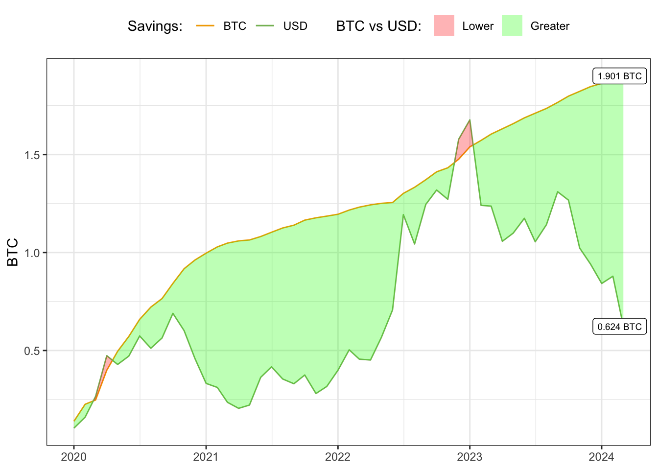
Here we compare the value of the savings in both cases expressed in BTC.

Show the code

last_cum_usd_savings <- result$cum_usd_savings_btc[nrow(result)]
last_cum_btc_savings <- result$cum_btc_savings_btc[nrow(result)]

result %>%
  ggplot() +
  geom_line(aes(date, cum_btc_savings_btc,  color = "btc")) +
  geom_line(aes(date, cum_usd_savings_btc, color = "usd")) +
  scale_color_manual(values = c(btc = mycol$btc, usd = mycol$usd), 
                     labels = c(btc = "BTC", usd = "USD"))+ 
  scale_fill_manual(values = c(`TRUE` = "green", `FALSE` = "red"),
                    labels = c(`TRUE` = "Greater", `FALSE` = "Lower"),
                    )+
  annotate(geom = "label",  size = 2.5,
           x = max(result$date)-10, y = last_cum_usd_savings, label = paste0(round(last_cum_usd_savings, 3), " BTC"))+
  annotate(geom = "label",  size = 2.5,
           x = max(result$date)-10, y = last_cum_btc_savings, label = paste0(round(last_cum_btc_savings, 3), " BTC"))+
  labs(fill = "BTC vs USD: ", color = "Savings: ", y = "BTC", x = NULL)+
  theme_bw()+
  theme(legend.position = "top")

Figure 4: Savings in both cases expressed in BTC.

2.2 Should I trade my BTC?

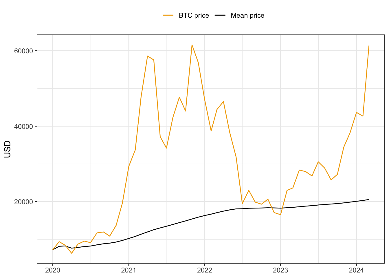
Let’s compute the mean price of the BTC that we convert at the beginning of the month.

Show the code

# Initialize 
result$mean_price <- 0
result$mean_price[1] <- result$btc_price[1]
for(i in 2:nrow(result)){
  # Compute the total btc converted 
  btc_weight <- result$btc_amount[1:i]
  # BTC mean price 
  btc_price <- result$btc_price[1:i]
  # Total btc 
  btc_sum_weights <- sum(btc_weight)
  result$mean_price[i] <- sum(btc_weight*btc_price)/btc_sum_weights
}

ggplot()+
  geom_line(data = result, aes(date, mean_price, color = "mean_price"))+
  geom_line(data = result, aes(date, btc_price, col = "btc_price"))+
  scale_color_manual(values = c(mean_price = "black", btc_price = mycol$btc),
                     labels = c(usd = "Savings USD", 
                                mean_price = "Mean price", 
                                btc_price = "BTC price"))+
  theme_bw()+
  theme(legend.position = "top")+
  labs(color = NULL, linetype = NULL, y = "USD", x = NULL)

Figure 5: BTC price and mean conversion price.

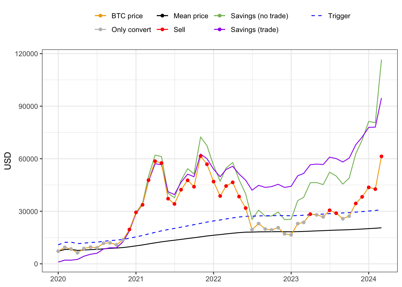
2.3 Fixed trading strategy

Let’s consider a simple trading strategy, where we sell a certain amount of our saved BTC if some conditions are met. Let’s imagine a reasonable setup for example: at the beginning of the month, when we convert our income, we will sell 5% of our savings if the price at the beginning of that is 50% greater than our average price.

Show the code

df_simple <- result
perc_sell <- 0.05 # 5%
threshold <- df_simple$mean_price*1.5 # 50% 
# =======================
df_simple$trade <- "buy"
df_simple$gain <- 0
df_simple$btc_sold <- 0
for(i in 1:nrow(df_simple)){
  # Compute the net btc saved
  btc_savings <- sum(df_simple$btc_savings[1:i]) - sum(df_simple$btc_sold[1:i])
  # Evaluate sell condition
  if (btc_savings > 0) {
    sell_condition <- df_simple$btc_price[i] > threshold[i]
    if (sell_condition) {
      # Compute the amount to be sold 
      btc_sell_amount <- btc_savings*perc_sell
      # Update trade variable 
      df_simple$trade[i] <- "sell"
      # Update capital gains
      df_simple$gain[i] <- btc_sell_amount*df_simple$btc_price[i]
      # Update btc sold 
      df_simple$btc_sold[i] <- btc_sell_amount
    }
  } else {
    sell_condition <- FALSE
  }
}
# Compute cumulated net saved btc 
df_simple$cum_btc_savings_btc <-  cumsum(df_simple$btc_savings - df_simple$btc_sold)
# Compute cumulated capital gain 
df_simple$cum_gain <- cumsum(df_simple$gain)

ggplot()+
  geom_line(data = result, aes(date, cum_btc_savings_btc*btc_price, color = "usd"))+
  geom_line(data = df_simple, aes(date, mean_price, color = "mean_price"))+
  geom_line(data = df_simple, aes(date, threshold, linetype = "threshold"), color = "blue")+
  geom_line(data = df_simple, aes(date, cum_btc_savings_btc*btc_price + cum_gain, col = "usd_trade"))+
  geom_line(data = df_simple, aes(date, btc_price, col = "btc_price"))+
  geom_point(data = df_simple, aes(date, btc_price, color = trade))+
  scale_linetype_manual(values = c(threshold = "dashed"), labels = c(threshold = "Trigger"))+
  scale_color_manual(values = c(usd = mycol$usd, mean_price = "black", 
                                usd_trade = "purple", btc_price = mycol$btc,
                                buy = "gray", sell = "red"),
                     labels = c(usd = "Savings (no trade)", 
                                mean_price = "Mean price", 
                                usd_trade = "Savings (trade)", 
                                btc_price = "BTC price",
                                buy = "Only convert", sell = "Sell"))+
  theme_bw()+
  theme(legend.position = "top")+
  labs(color = NULL, linetype = NULL, y = "USD", x = NULL)

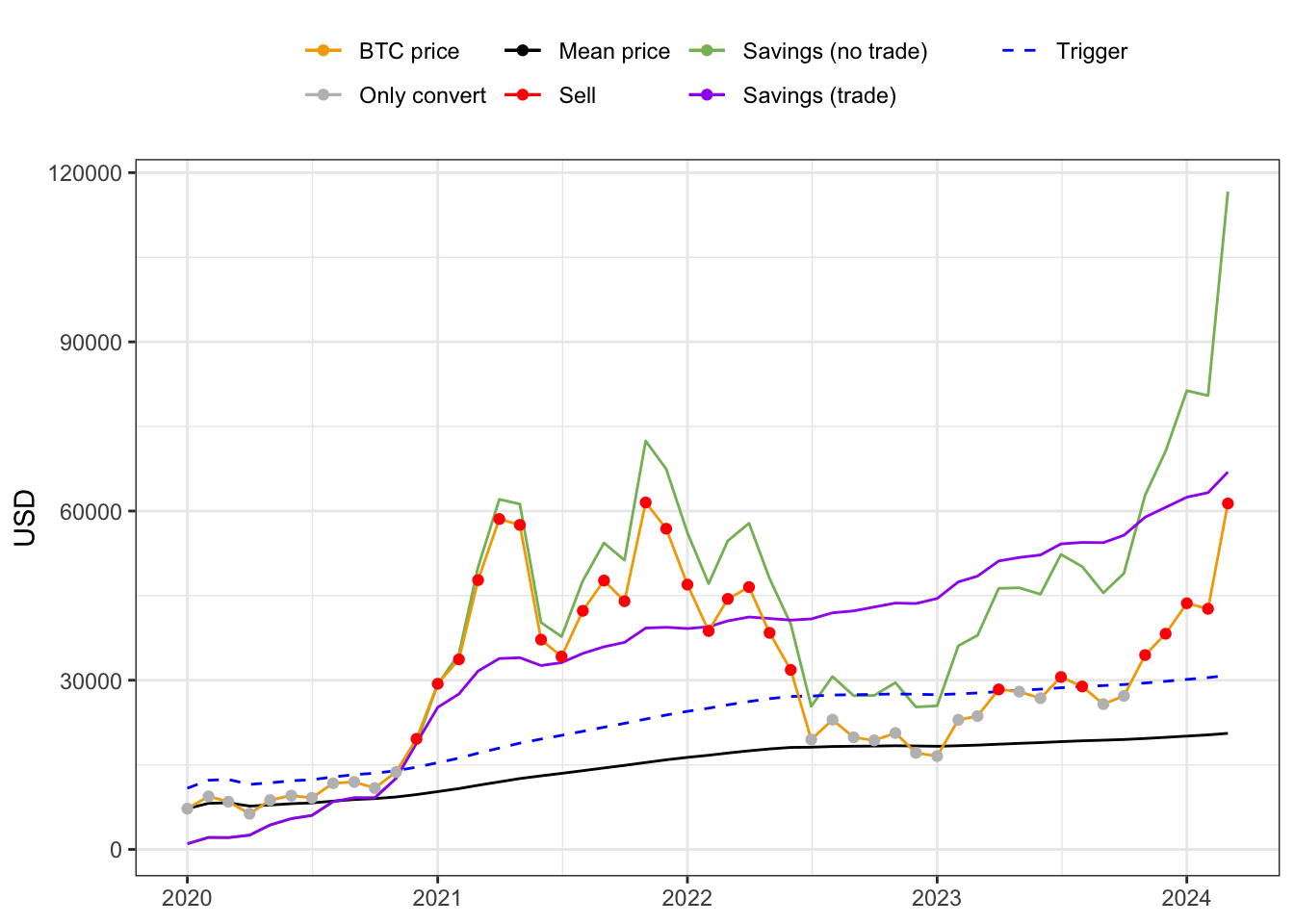
2.4 Volatility trading strategy

Let’s consider the volatility of BTC price computed randomly at the expenses dates. The idea is to adapt the amount sold in our strategy with respect to the volatility. For example, if the price is above the trigger, and so we have to sell a certain amount, we want to sell adapting the amount with respect to the volatility in the past 5 months. In practice, in the month $i$-th, we compute the volatility of the expenses in the past $j = i-5, \dots, i-1$ months, i.e. $\sigma_j$. Then, we normalize the values in order to have a number in $(0,1)$. In this way the percentage of savings that we are going to sell in the month $i$-th is given by $q_{i-1} = \sigma_{i-1}/\sum_{j}\sigma_j$.

Show the code

df_vol <- result
threshold <- df_vol$mean_price*1.5 # 50% 
# =======================
df_vol$trade <- "buy"
df_vol$gain <- 0
df_vol$btc_sold <- 0
for(i in 6:nrow(df_vol)){
  # Compute the net btc saved
  btc_savings <- sum(df_vol$btc_savings[1:i]) - sum(df_vol$btc_sold[1:i])
  # Evaluate sell condition
  if (btc_savings > 0) {
    sell_condition <- df_vol$btc_price[i] > threshold[i]
    if (sell_condition) {
      # Compute the percentage of savings to sell 
      sum_sigma <- sum(df_vol$btc_vol[(i-5):(i-1)])
      perc_sell <- df_vol$btc_vol[i-1]/sum_sigma
      # Compute the amount to be sold 
      btc_sell_amount <- btc_savings*perc_sell
      # Update trade variable 
      df_vol$trade[i] <- "sell"
      # Update capital gains
      df_vol$gain[i] <- btc_sell_amount*df_vol$btc_price[i]
      # Update btc sold 
      df_vol$btc_sold[i] <- btc_sell_amount
    }
  } else {
    sell_condition <- FALSE
  }
}
# Compute cumulated net saved btc 
df_vol$cum_btc_savings_btc <-  cumsum(df_vol$btc_savings - df_vol$btc_sold)
# Compute cumulated capital gain 
df_vol$cum_gain <- cumsum(df_vol$gain)

ggplot()+
  geom_line(data = result, aes(date, cum_btc_savings_btc*btc_price, color = "usd"))+
  geom_line(data = df_vol, aes(date, mean_price, color = "mean_price"))+
  geom_line(data = df_vol, aes(date, threshold, linetype = "threshold"), color = "blue")+
  geom_line(data = df_vol, aes(date, cum_btc_savings_btc*btc_price + cum_gain, col = "usd_trade"))+
  geom_line(data = df_vol, aes(date, btc_price, col = "btc_price"))+
  geom_point(data = df_vol, aes(date, btc_price, color = trade))+
  scale_linetype_manual(values = c(threshold = "dashed"), labels = c(threshold = "Trigger"))+
  scale_color_manual(values = c(usd = mycol$usd, mean_price = "black", 
                                usd_trade = "purple", btc_price = mycol$btc,
                                buy = "gray", sell = "red"),
                     labels = c(usd = "Savings (no trade)", 
                                mean_price = "Mean price", 
                                usd_trade = "Savings (trade)", 
                                btc_price = "BTC price",
                                buy = "Only convert", sell = "Sell"))+
  theme_bw()+
  theme(legend.position = "top")+
  labs(color = NULL, linetype = NULL, y = "USD", x = NULL)

2.5 Monthly Outcome Summary

At the end of each month, we assess the impact of Bitcoin’s volatility on overall expenses and remaining balances. This summary offers a clear picture of how well the initial monthly conversion managed to cover the expenses under various price scenarios. Key outcomes to observe include:

Surplus or Shortfall: If Bitcoin’s price rose during the month, there may be leftover funds; if it fell, there could be a shortfall, affecting the ability to cover all expenses.
Average Purchasing Power: A comparison of the average value of each conversion throughout the month against the initial conversion rate can show how favorable or unfavorable the month’s volatility was for daily expenses.

This summary encapsulates the monthly effects of volatility on an individual’s financial situation and underscores the challenges of using Bitcoin for consistent spending.

Code

cum_savings <- result$cum_btc_savings_btc*result$btc_price 
cum_savings_simple <- df_simple$cum_btc_savings_btc*df_simple$btc_price + df_simple$cum_gain
cum_savings_vol <- df_vol$cum_btc_savings_btc*df_vol$btc_price + df_vol$cum_gain

tibble(
  sd_notrade = sd(diff(log(cum_savings))),
  sd_simple = sd(diff(log(cum_savings_simple))),
  sd_vol = sd(diff(log(cum_savings_vol)))
) %>%
  mutate_all(~paste0(format(.x*100, digits=4), " %")) %>%
  knitr::kable(col.names = c("Std. Deviation (No trade)", 
                             "Std. Deviation (Simple)", 
                             "Std. Deviation (Volatility)"))

Std. Deviation (No trade)	Std. Deviation (Simple)	Std. Deviation (Volatility)
23.41 %	18.82 %	15.69 %

3 Conclusions

The volatility of Bitcoin poses unique considerations for individuals relying on it for monthly spending. Beyond our initial analysis, other factors could significantly affect outcomes, such as:

Transaction Fees: Bitcoin transaction fees can add up, especially with frequent conversions, impacting the effective value received in each transaction.
Timing of Conversions: Some individuals may try to time conversions to align with higher prices, but this strategy may not be feasible for essential expenses.
Alternative Stable Assets: Using stablecoins or partially diversifying income with other assets could offer more stability for daily spending needs. However, it is subject to the inflation of US Dollar, that, in the long run, lead to a loss if we measure the purchasing power in BTC.

These considerations highlight both the challenges and potential strategies for managing Bitcoin as a primary financial asset, emphasizing the need for adaptable approaches to maintain purchasing power amid price fluctuations.

Citation

BibTeX citation:

@online{sartini2024,
  author = {Sartini, Beniamino},
  title = {Bitcoin Is Volatile?},
  date = {2024-11-10},
  url = {https://cryptoverser.org/articles/bitcoin-expenses/bitcoin-expenses.html},
  langid = {en}
}

For attribution, please cite this work as:

Sartini, Beniamino. 2024. “Bitcoin Is Volatile?” November 10, 2024. https://cryptoverser.org/articles/bitcoin-expenses/bitcoin-expenses.html.