Bitcoin and Metcalfe Law

Moving average function

# Simple Moving Average
SMA <- function(x = NULL, n = 10, fun = mean, na.rm = TRUE){
  N <- length(x)
  y <- rep(NA_integer_, N)
  for(i in n:N){
    y[i] <- fun(x[(i - n + 1):i], na.rm = na.rm)
  }
  return(y)
}

Show the Custom theme

# Custom theme 
custom_theme <- 
theme(axis.title  = element_text(face = "bold"), 
        plot.title  = element_text(face = "bold"),
        axis.line = element_line(),
        axis.text.x = element_text(angle = 0, face = "bold", size = 7), 
        axis.text.y = element_text(face = "bold"), 
        axis.title.x = element_text(face = "bold",size = 10),
        axis.title.y = element_text(face = "bold", size = 10),
        plot.subtitle = element_text(face = "italic"),
        plot.caption = element_text(face = "italic"),
        panel.grid.minor.x = element_blank(),
        panel.grid.minor.y = element_blank(),
        panel.grid.major.x = element_blank(),
        panel.grid.major.y = element_line(
          color = "black", linetype = "dashed", linewidth = 0.05),
        panel.border = element_blank(),
        strip.background = element_blank(),
        panel.background = element_blank(),
        strip.text = element_text(angle = 0, face = "bold", size = 7), 
        legend.title = element_text(face = "bold", size = 11),
        legend.text = element_text(face = "italic", size = 10),
        legend.box.background = element_rect(),
        legend.position = "top") 

1 Disclaimer

This work examine the paper Peterson (2018) and tries to reproduce its results considering the Bitcoin price from 2017-04-08 up to 2023-05-23.

2 On-chain analysis

Show the code

BTC_chain$SMA_active_addresses <- SMA(BTC_chain$active_addresses, n = 30)
BTC_chain$SMA_new_addresses <- SMA(BTC_chain$new_addresses, n = 30)

ggplot()+
  geom_line(data = BTC_chain, color = "#FF9416",
            aes(Date, SMA_active_addresses/1000)) +
  geom_line(data = BTC_chain, color = "#FF7116",
            aes(Date, SMA_new_addresses/1000)) +
  geom_label(data = tail(BTC_chain, 1), color = "black", size = 2,
             aes(Date-20, SMA_new_addresses/1000, label = "New Addresses")) +
  geom_label(data = tail(BTC_chain, 1), color = "black", size = 2,
             aes(Date-20, SMA_active_addresses/1000, label = "Active Addresses")) +
  labs(title = "30 days MA for Bitcoin wallets", caption = "Source: Cryptocompare",
       x = NULL, y = "30 Days SMA (thousands)") + 
  custom_theme + 
  scale_x_date(breaks = seq.Date(as.Date("2017-04-08"), Sys.Date(), 250)) +
  scale_y_continuous(breaks = seq(0, 2000, 100))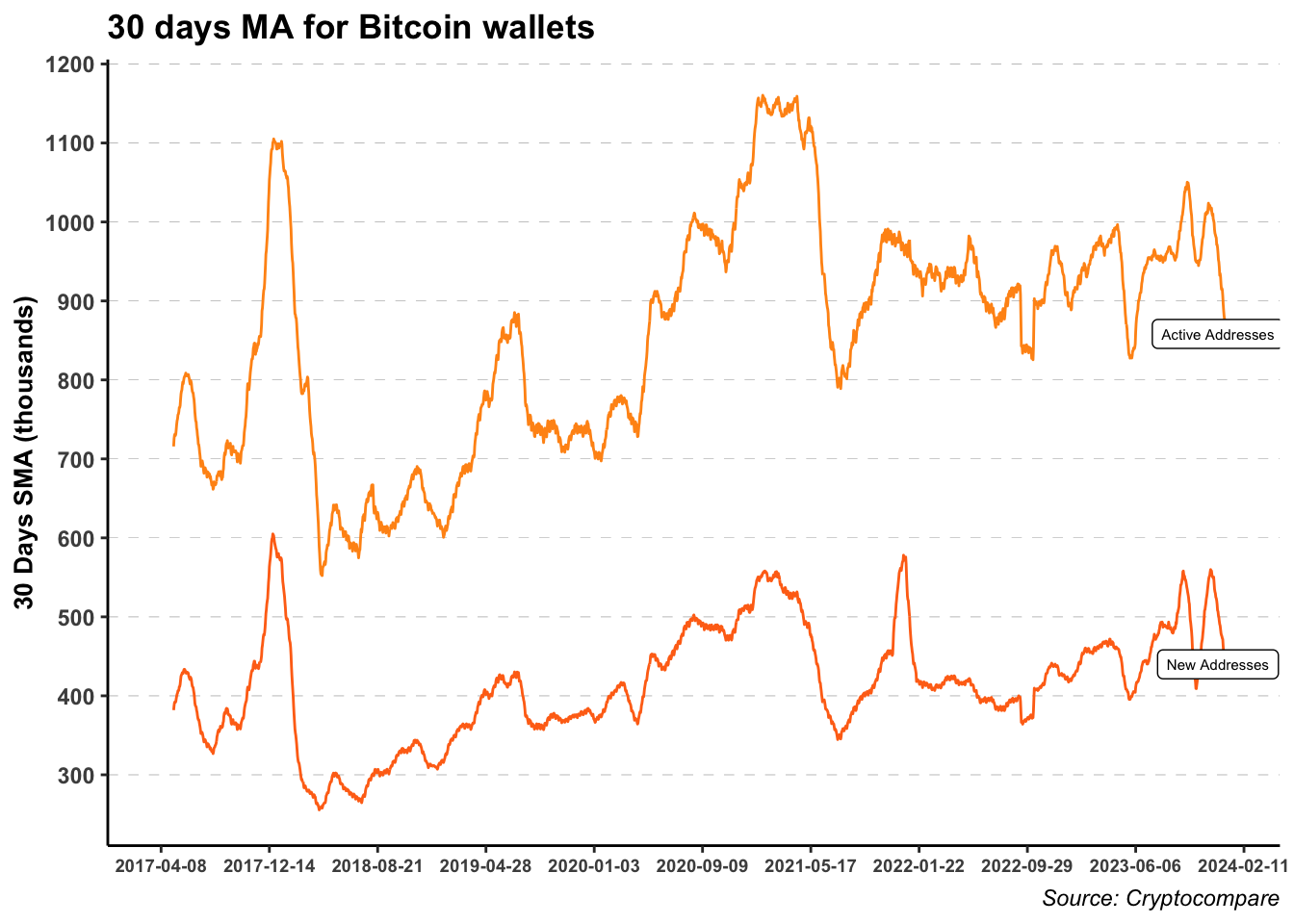

Show the code

ggplot(BTC_chain)+
  geom_line(aes(Date, transaction_count/active_addresses*100), color = "#FF9416" )+
  custom_theme + 
  labs(title = "Ratio between number of daily transactions and active wallets", 
       caption = "Source: Cryptocompare", x = NULL, y = NULL) + 
  scale_x_date(breaks = seq.Date(as.Date("2017-04-08"), Sys.Date(), 365))+
  scale_y_continuous(breaks = seq(0, 400, 20), labels = paste0(seq(0, 400, 20), "%"))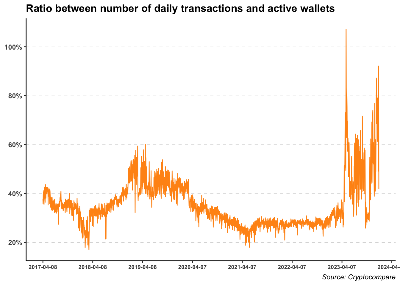

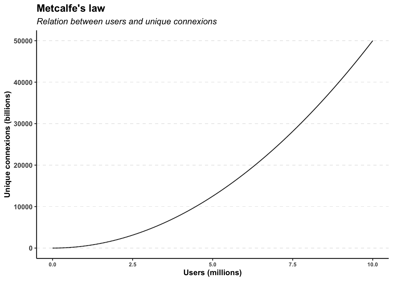
3 Metcalfe law

Metcalfe’s Law applied to Bitcoin states that the value of a network is proportional to the square of its user base. In the context of Bitcoin, this means that as more people join and use the cryptocurrency, its overall value increases exponentially. Bitcoin operates on a decentralized peer-to-peer network, allowing users to send and receive payments without intermediaries. The reasoning behind the use of this model is that the more participants in the Bitcoin network, the greater should be the potential for transactions and the network’s utility.

The law is named for Robert Metcalfe and first proposed in 1980, albeit not in terms of users, but rather of “compatible communicating devices”, such as telephones. It later became associated with users on the Ethernet.

Metcalfe’s Law is related to the fact that the number of unique possible connections $C_n$ in a network of $n$ nodes. It can be expressed mathematically as a number asymptotically proportional to $n^2$.

$$C_n=\frac{n(n-1)}{2}\underset{n\to \mathrm{\infty }}{\propto }{n}^2$$

Show the code

n_grid <- seq(1, 10000000, 100)
C_n <- function(n){n*(n-1)*0.5}
ggplot()+
  geom_line(aes(n_grid/1000000, C_n(n_grid)/1000000000)) +
  custom_theme +
  labs(x = "Users (millions)", y = "Unique connexions (billions)", title = "Metcalfe's law", 
       subtitle = "Relation between users and unique connexions")

Metcalfe himself, however, applied a proportionality factor $A$ that he acknowledged could decrease over time. The law was originally designed to identify the number of users $n$ at which the costs $C$ for network implementation would be recovered (originally applied to telephone networks). In mathematical terms:

$$M(n)=nC=A\frac{n(n-1)}{2}$$

4 Reed’s Law Network Model

Reed’s law is the assertion that the utility of large networks, particularly social networks, can scale exponentially with the size of the network. The reason for this is that the number of possible sub-groups of network participants is:

$$C_n=2^n-n-1$$ This grows much more rapidly than either the number of users $n$, or the number of possible pair connections $n^2$.

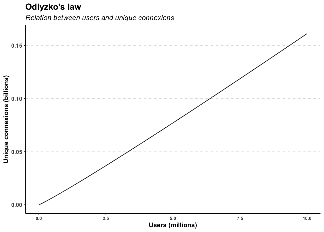
5 Odlyzko’s Law Network Model

Briscoe et. al. [2006] believe that Metcalfe’s and Reed’s laws are too optimistic in their values. They argue, without mathematical proof, the growth rate of the network must decrease as subsequent members join because the most valuable links are likely to be formed first. This parallels the concept of “diminishing returns” central to neo classical economics. Such diminishing incremental value was modeled:

$$n\text{log}(n)$$

Show the code

n_grid <- seq(1, 10000000, 100)
C_n <- function(n){n*log(n)}
ggplot()+
  geom_line(aes(n_grid/1000000, C_n(n_grid)/1000000000))+
  custom_theme +
  labs(x = "Users (millions)", y = "Unique connexions (billions)", title = "Odlyzko's law", 
       subtitle = "Relation between users and unique connexions")

6 Bitcoin inflation

Code

df_bitcoin_supply <- BitcoinSupply(end_date = "2045-01-01", quiet = TRUE)
df_bitcoin_halving <- df_bitcoin_supply[df_bitcoin_supply$Halving,]
y_breaks <- seq.int(min(df_bitcoin_supply$Supply), max(df_bitcoin_supply$Supply), by = 2000000)
ggplot()+
  geom_line(data = df_bitcoin_supply, aes(Date, Supply)) +
  geom_point(data = df_bitcoin_halving, aes(Date, Supply), color = "red") +
  geom_segment(data = df_bitcoin_halving, color = "red", linetype = "dashed",
               aes(x = Date, xend = Date, y = 0, yend = Inf)) +
  geom_label(data = df_bitcoin_halving, color = "red", linetype = "dashed", size = 3,
             aes(x = Date, y = 0, label = paste0("Halving ", N_Halving))) +
  scale_y_continuous(breaks = y_breaks, labels = as.character(y_breaks)) +
  custom_theme +
  labs(x = "Time (days)", y = "Total supply (BTC)", title = "Bitcoin monetary supply")

7 Bitcoin Equilibrium Price with Network Models

Code

BTC <- left_join(select(BTC_daily, Date, Symbol, Price = "Close"), 
                 select(BTC_chain, 
                        Date, active_addresses, transaction_count, current_supply, hashrate), 
                 by = "Date")

index_date <- seq.Date(as.Date("2017-01-01"), as.Date("2024-01-01"), by = "1 month")

BTC <- filter(BTC, Date %in% index_date)

BTC$log_price <- log(BTC$Price)

# Network Value 
BTC$metcalfe <- BTC$active_addresses*(BTC$active_addresses-1)/2
BTC$value_metcalfe <- log(BTC$metcalfe*(1/BTC$current_supply))

BTC$odlyzko <- BTC$active_addresses*log(BTC$active_addresses)
BTC$value_odlyzko <- log(BTC$odlyzko*(1/BTC$current_supply))

BTC <- na.omit(BTC)

metcalfe_model_BTC <- lm(log_price ~ value_metcalfe, data = BTC) 
odlyzko_model_BTC <- lm(log_price ~ value_odlyzko , data = BTC) 
mixed_model_BTC <- lm(log_price ~ value_metcalfe + value_odlyzko, data = BTC) 

BTC %>%
  mutate(fitted_metcalfe = predict(metcalfe_model_BTC),
         fitted_odlyzko = predict(odlyzko_model_BTC), 
         fitted_mixed = predict(mixed_model_BTC)) %>%
  ggplot() +
  geom_line(aes(Date, fitted_metcalfe, color = "metcalfe"))+
  geom_line(aes(Date, fitted_mixed, color = "mixed"), alpha = 0.8)+
  #geom_line(aes(Date, fitted_odlyzko, color = "odlyzko"), alpha = 0.8)+
  geom_line(aes(Date, log_price, color = "log_price"))+
  scale_color_manual(values = c(metcalfe = "red", odlyzko = "purple", 
                                mixed = "green", log_price = "#FF9416"), 
                     labels = c(metcalfe = "Metcalfe", odlyzko = "Odlyzko", 
                                mixed = "Mixed", log_price = "Log-price" ))+
  scale_y_continuous(breaks = round(seq(min(BTC$log_price), max(BTC$log_price), length.out=10),2))+
  scale_x_date(breaks = seq.Date(min(BTC$Date), max(BTC$Date), length.out = 10))+
  theme(axis.title  = element_text(face = "bold"), 
        plot.title  = element_text(face = "bold"),
        axis.line = element_line(),
        axis.text.x = element_text(angle = 0, face = "bold", size = 7), 
        axis.text.y = element_text(face = "bold"), 
        axis.title.x = element_text(face = "bold",size = 10),
        axis.title.y = element_text(face = "bold", size = 10),
        plot.subtitle = element_text(face = "italic"),
        plot.caption = element_text(face = "italic"),
        panel.grid.minor.x = element_blank(),
        panel.grid.minor.y = element_blank(),
        panel.grid.major.x = element_blank(),
        panel.grid.major.y = element_line(color = "#FF9416", linetype = "dashed", linewidth = 0.1),
        panel.border = element_blank(),
        strip.background = element_blank(),
        panel.background = element_blank(),
        strip.text = element_text(angle = 0, face = "bold", size = 7), 
        legend.title = element_text(face = "bold", size = 11),
        legend.text = element_text(face = "italic", size = 10),
        legend.box.background = element_rect(),
        legend.position = "top") +
  labs(color="Model: ")+
  ggtitle("Networks models for Bitcoin log-price") +
  labs(x ="", y="Log-price", caption = "")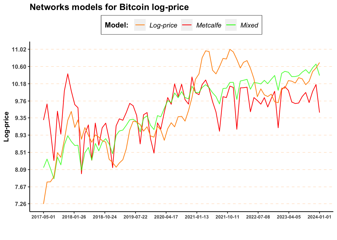

Code

BTC %>%
  mutate(fitted_metcalfe = predict(metcalfe_model_BTC) %>% exp(),
         fitted_odlyzko = predict(odlyzko_model_BTC)%>% exp(), 
         fitted_mixed = predict(mixed_model_BTC)%>% exp()) %>%
  ggplot() +
  geom_line(aes(Date, fitted_metcalfe, color = "metcalfe"))+
  geom_line(aes(Date, fitted_mixed, color = "mixed"), alpha = 0.8)+
  geom_line(aes(Date, fitted_odlyzko, color = "odlyzko"), alpha = 0.8)+
  geom_line(aes(Date, log_price%>% exp(), color = "price"))+
  scale_color_manual(values = c(metcalfe = "red", odlyzko = "purple", mixed = "green", 
                                log_price = "#FF9416"), 
                     labels = c(metcalfe = "Metcalfe", odlyzko = "Odlyzko", mixed = "Mixed",
                                price = "Price" ))+
  scale_y_continuous(breaks = round(seq(min(exp(BTC$log_price)), max(exp(BTC$log_price)), length.out=10),2))+
  scale_x_date(breaks = seq.Date(min(BTC$Date), max(BTC$Date), length.out = 10))+
  theme(axis.title  = element_text(face = "bold"), 
        plot.title  = element_text(face = "bold"),
        axis.line = element_line(),
        axis.text.x = element_text(angle = 0, face = "bold", size = 7), 
        axis.text.y = element_text(face = "bold"), 
        axis.title.x = element_text(face = "bold",size = 10),
        axis.title.y = element_text(face = "bold", size = 10),
        plot.subtitle = element_text(face = "italic"),
        plot.caption = element_text(face = "italic"),
        panel.grid.minor.x = element_blank(),
        panel.grid.minor.y = element_blank(),
        panel.grid.major.x = element_blank(),
        panel.grid.major.y = element_line(color = "#FF9416", linetype = "dashed", linewidth = 0.1),
        panel.border = element_blank(),
        strip.background = element_blank(),
        panel.background = element_blank(),
        strip.text = element_text(angle = 0, face = "bold", size = 7), 
        legend.title = element_text(face = "bold", size = 11),
        legend.text = element_text(face = "italic", size = 10),
        legend.box.background = element_rect(),
        legend.position = "top") +
  labs(color="Model: ")+
  ggtitle("Networks models for Bitcoin log-price") +
  labs(x ="", y="Log-price", caption = "")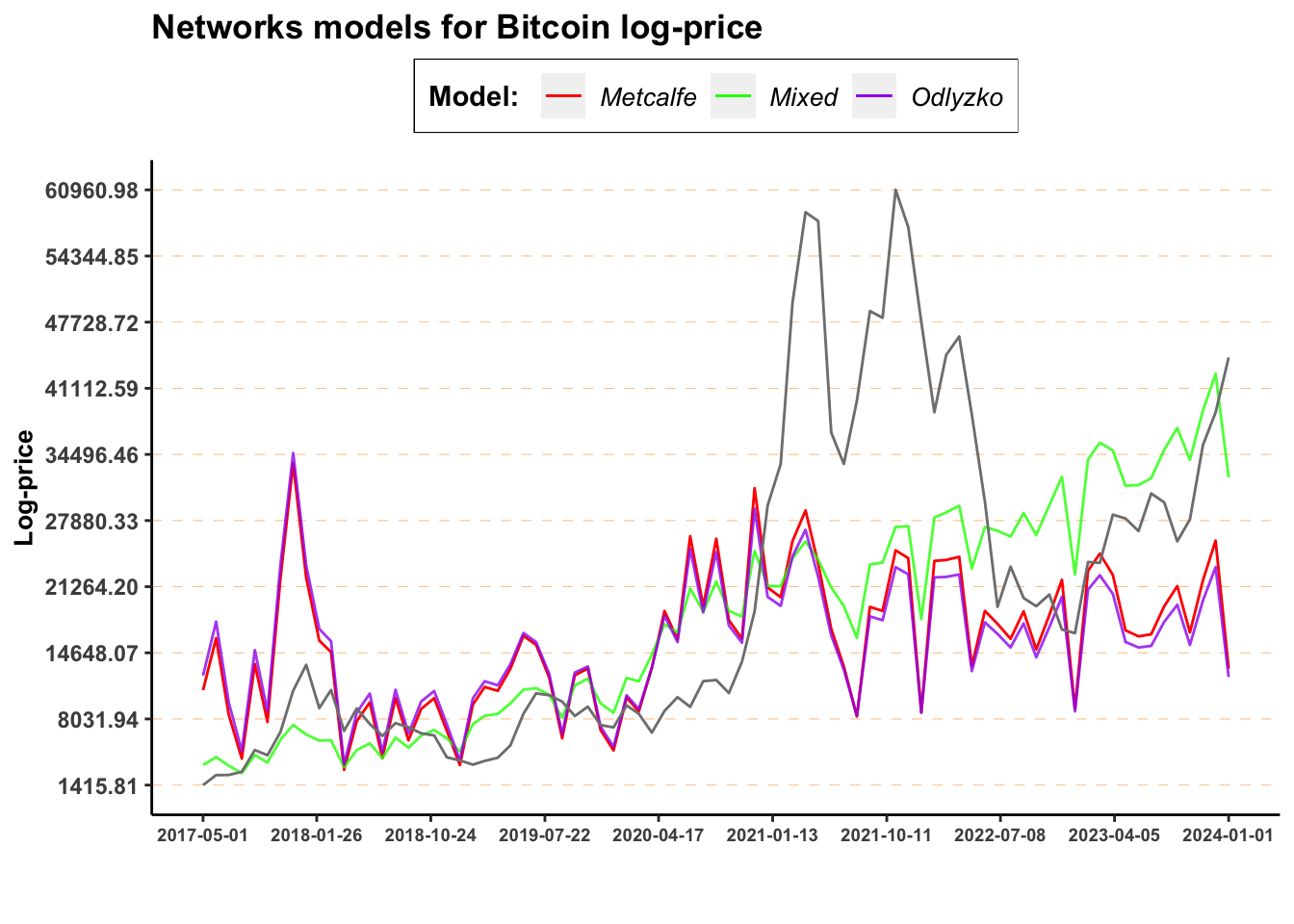

Code

bind_rows(
  bind_cols(Model = "Metcalfe", 
          broom::tidy(summary(metcalfe_model_BTC))),
  bind_cols(Model = "Odlyzko", 
          broom::tidy(summary(odlyzko_model_BTC))),
  bind_cols(Model = "Mixed", 
          broom::tidy(summary(mixed_model_BTC))) 
) %>%
  knitr::kable() %>%
  kableExtra::kable_classic_2()

Model	term	estimate	std.error	statistic	p.value
Metcalfe	(Intercept)	-2.502297	1.8897676	-1.324130	0.1892784
Metcalfe	value_metcalfe	1.221037	0.1911761	6.386976	0.0000000
Odlyzko	(Intercept)	10.540437	0.2006525	52.530812	0.0000000
Odlyzko	value_odlyzko	2.133695	0.3926249	5.434436	0.0000006
Mixed	(Intercept)	-142.473848	14.1333207	-10.080706	0.0000000
Mixed	value_metcalfe	14.203414	1.3118594	10.826934	0.0000000
Mixed	value_odlyzko	-25.499556	2.5644609	-9.943437	0.0000000

Code

bind_rows(
  bind_cols(Model = "Metcalfe", 
          broom::glance(summary(metcalfe_model_BTC))),
  bind_cols(Model = "Odlyzko", 
          broom::glance(summary(odlyzko_model_BTC))),
  bind_cols(Model = "Mixed", 
          broom::glance(summary(mixed_model_BTC))) 
) %>%
  knitr::kable() %>%
  kableExtra::kable_classic_2()

Model	r.squared	adj.r.squared	sigma	statistic	p.value	df	df.residual	nobs
Metcalfe	0.3405316	0.3321839	0.7398415	40.79346	0e+00	1	79	81
Odlyzko	0.2721114	0.2628977	0.7772740	29.53310	6e-07	1	79	81
Mixed	0.7091764	0.7017194	0.4944504	95.10191	0e+00	2	78	81

References

Peterson, Timothy. 2018. “Metcalfe’s Law as a Model for Bitcoin’s Value.” Alternative Investment Analyst Review 7 (2): 9–18. https://doi.org/10.2139/ssrn.3078248.

Citation

BibTeX citation:

@online{sartini2024,
  author = {Sartini, Beniamino},
  title = {Bitcoin and {Metcalfe} {Law}},
  date = {2024-06-19},
  url = {https://cryptoverser.org/articles/bitcoin-metcalfe/bitcoin-metcalfe.html},
  langid = {en}
}

For attribution, please cite this work as:

Sartini, Beniamino. 2024. “Bitcoin and Metcalfe Law.” June 19, 2024. https://cryptoverser.org/articles/bitcoin-metcalfe/bitcoin-metcalfe.html.