The seasonal effect on Bitcoin (BTC) returns refers to the observed patterns and trends that occur during specific periods within a year. Researchers have found evidence suggesting the presence of seasonality in BTC returns, indicating recurring patterns that investors and traders can potentially exploit. These patterns can help inform investment strategies and improve market timing.

Code

library(tidyverse)
library(DT)
BTCUSDT <- read_csv("BTCUSDT-spot-1d.csv")
label_days <- c("Monday", "Tuesday", "Wednesday", "Thursday", "Friday", "Saturday", "Sunday")

Code

date_to_plot <- max(BTCUSDT$date)
date_from_plot <- date_to_plot - lubridate::days(60)
# Candle chart plot of last 60 days 
BTCUSDT %>%
  filter(date >= date_from_plot & date <= date_to_plot) %>%
  ggplot()+
  binancer::geom_candlechart(aes(x = date, close = close, open = open, low = low, high = high))+
  theme_bw()+
  theme(legend.position = "none")+
  labs(x = NULL)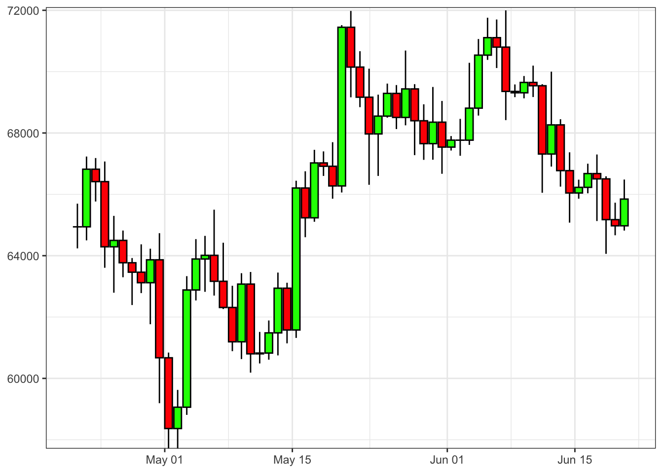

One well-known seasonal effect is the January effect, where BTC returns tend to be above average during the month of January. This phenomenon has been observed over multiple years, suggesting a consistent pattern. Another notable seasonal effect is the December effect, which indicates higher BTC returns during the month of December. Market activity during the holiday season and investor sentiment are factors that may contribute to this effect.

Code

# Compute cumulated return for each year 
df_years <- list()
df <- BTCUSDT
df$Year <- lubridate::year(df$date)
df$Year_ <- factor(df$Year, levels = c(min(df$Year):max(df$Year)), ordered = TRUE)
df$n <- solarr::number_of_day(df$date)
for(y in unique(df$Year)){
  df_y <- dplyr::filter(df, Year == y)
  df_y$Rt <- c(0, diff(log(df_y$close)))
  df_y$cum_ret <- cumprod(exp(df_y$Rt))
  df_years[[y]] <- df_y
}
df_years <- bind_rows(df_years)

x_breaks <- seq(1, 365, 40)
x_labels <- dplyr::filter(df, Year == 2020)[x_breaks,]$date
x_labels <- str_remove_all(as.Date(x_labels), "2020-")
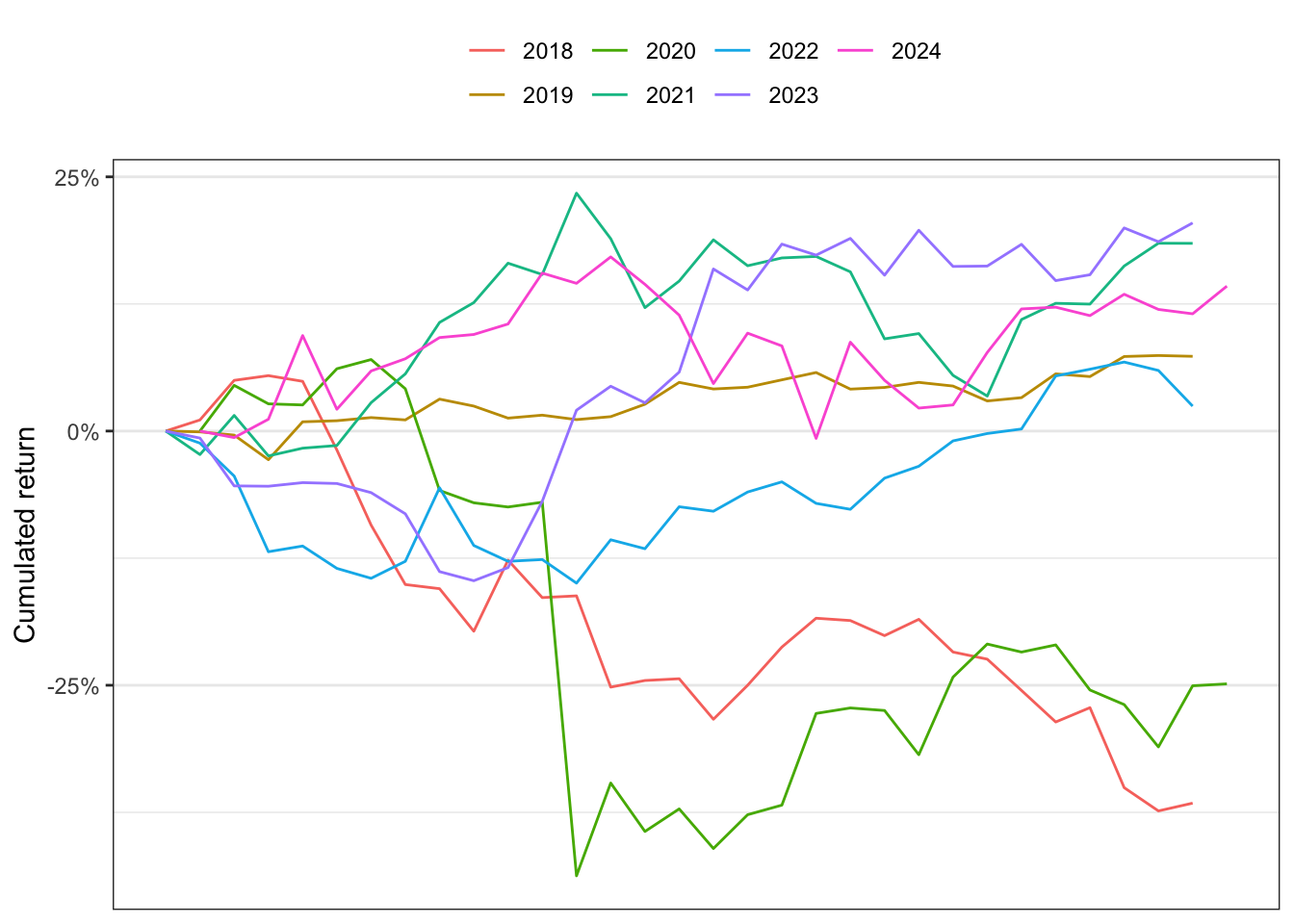
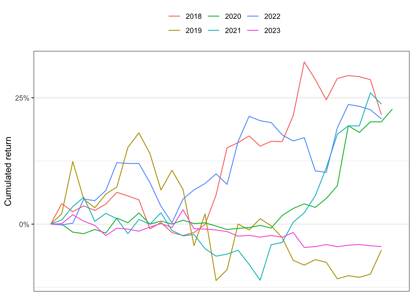
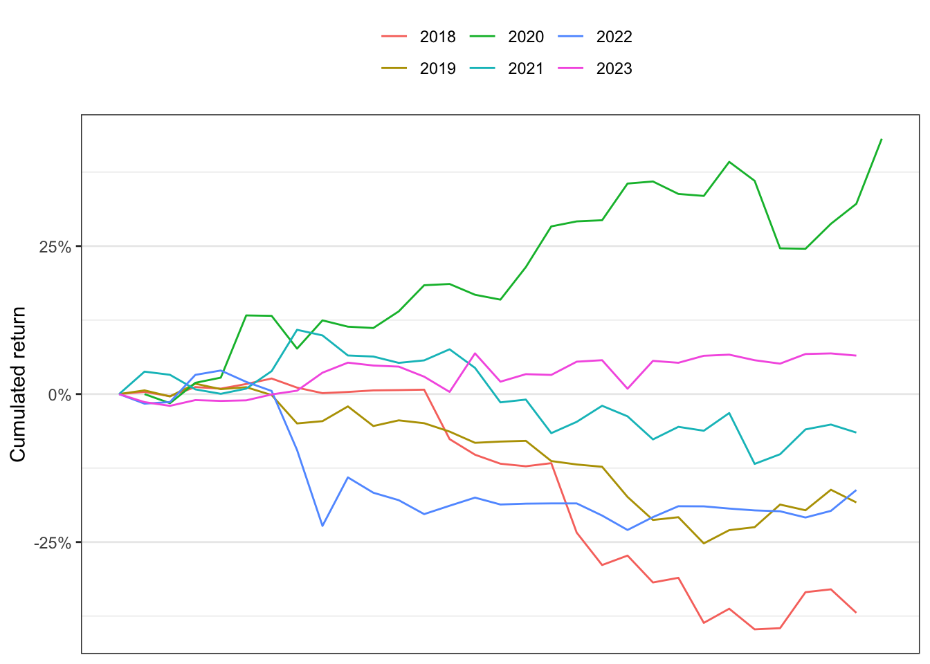
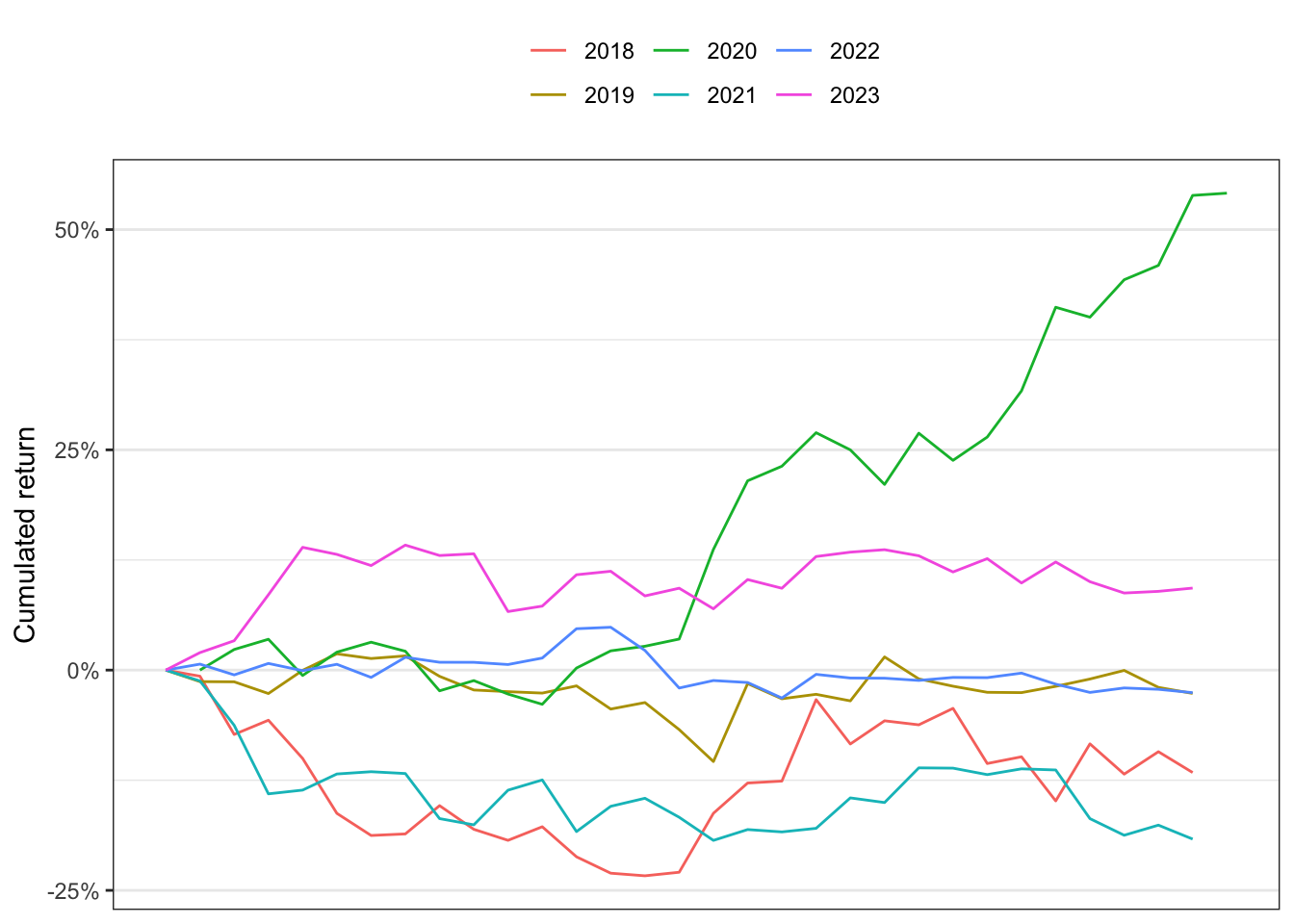
ggplot(df_years)+
  geom_line(aes(n, cum_ret, group = Year_, color = as.character(Year_)))+
  theme_bw()+
  theme(legend.position = "top")+
  scale_x_continuous(breaks = x_breaks, labels = x_labels)+
  scale_y_continuous(breaks = seq(0, 4, 0.5), labels = paste0((seq(0, 4, 0.5)-1)*100, "%"))+
  labs(color = NULL, y = "Cumulated return", x = NULL)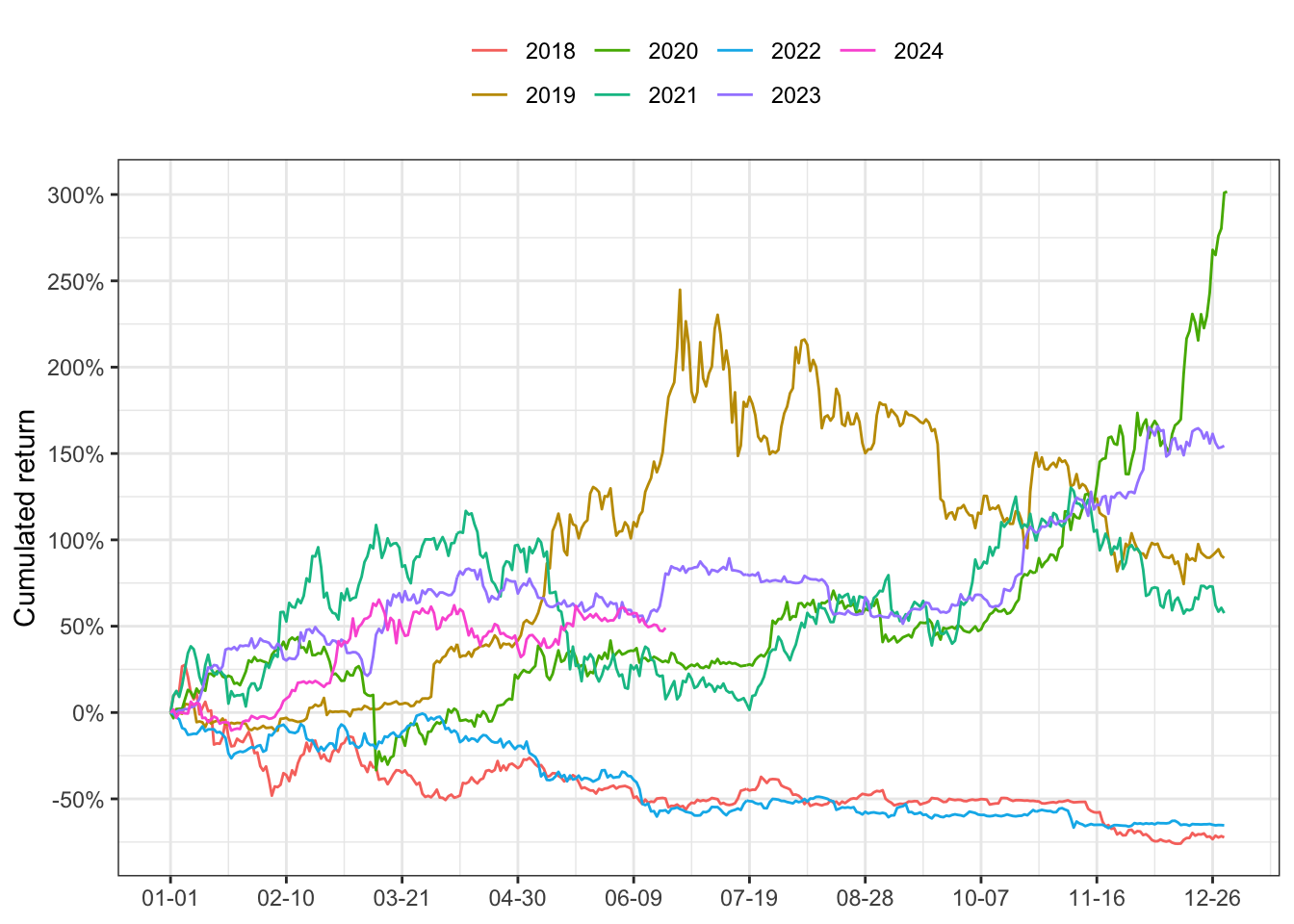

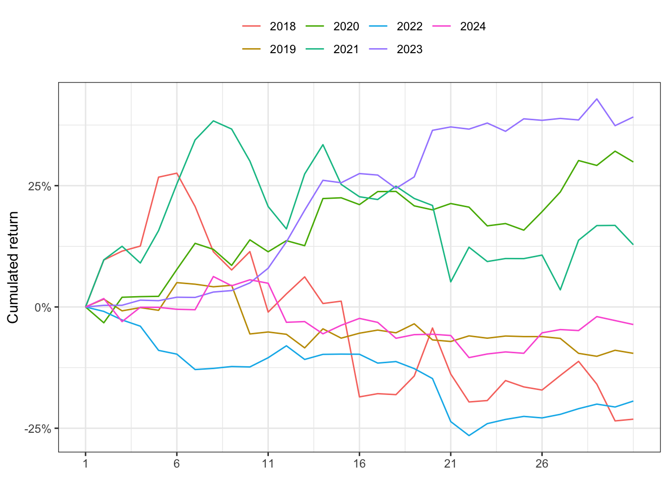
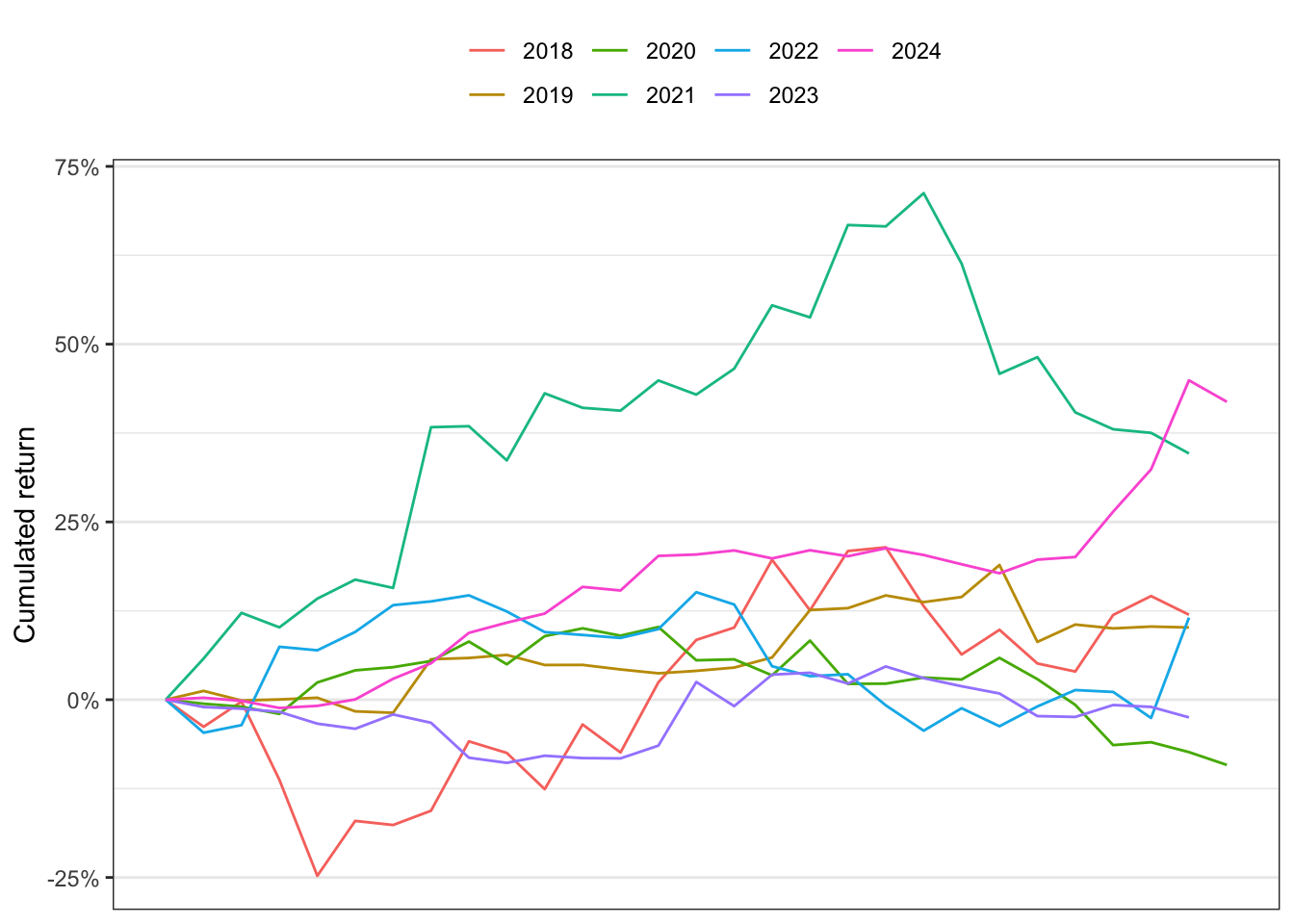
0.1 Monthly seasonality

Code

# Compute cumulated return for each year 
df_years <- list()
df <- BTCUSDT
df$Year <- lubridate::year(df$date)
df$Year_ <- factor(df$Year, levels = c(min(df$Year):max(df$Year)), ordered = TRUE)
df$Month <- lubridate::month(df$date)
df$Month_ <- factor(df$Month,
                    levels = c(1:12), 
                    labels = lubridate::month(1:12, label = TRUE),
                    ordered = TRUE)
df$Day <- lubridate::day(df$date)
df$n <- solarr::number_of_day(df$date)
k <- 1
for(y in unique(df$Year)){
  for(m in unique(df$Month)){
    df_y <- filter(df, Year == y & Month == m)
    df_y$Rt <- c(0, diff(log(df_y$close)))
    df_y$cum_ret <- cumprod(exp(df_y$Rt))
    df_years[[k]] <- df_y
    k <- k + 1
  }
}

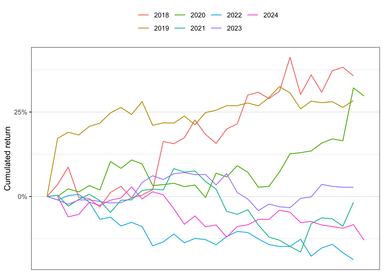
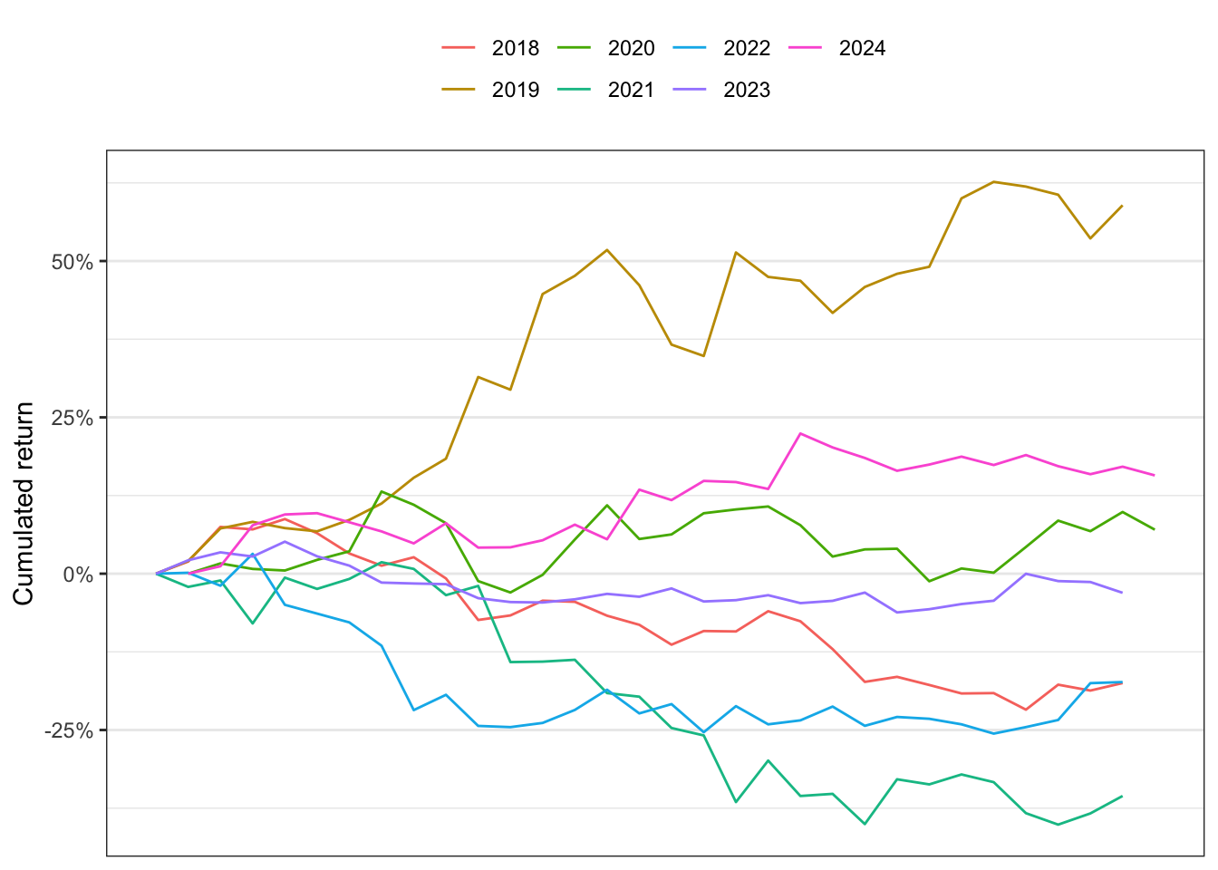
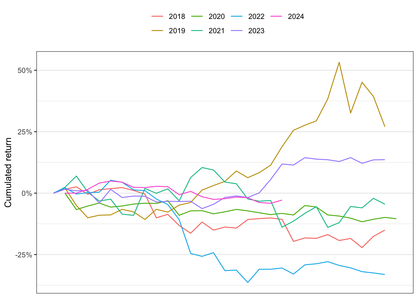
plot_cumret_month <- function(df_years, m = 1){
  
  df_years <- bind_rows(df_years)
  x_breaks <- seq(1, 30, 5)
  y_breaks <- seq(0, 2, 0.25)
  y_labels <- paste0((seq(0, 2, 0.25)-1)*100, "%")
  
  df_years %>%
    filter(Month == m) %>%
    ggplot()+
    geom_line(aes(n, cum_ret, group = Year_, color = as.character(Year_)))+
    theme_bw()+
    theme(legend.position = "top")+
    scale_x_continuous(breaks = x_breaks)+
    scale_y_continuous(breaks = y_breaks, labels = y_labels)+
    labs(color = NULL, y = "Cumulated return", x = NULL)
}

Code

plot_cumret_month(df_years, m = 1)

Code

plot_cumret_month(df_years, m = 2)

Code

plot_cumret_month(df_years, m = 3)

Code

plot_cumret_month(df_years, m = 4)

Code

plot_cumret_month(df_years, m = 5)

Code

plot_cumret_month(df_years, m = 6)

Code

plot_cumret_month(df_years, m = 7)

Code

plot_cumret_month(df_years, m = 8)

Code

plot_cumret_month(df_years, m = 9)

Code

plot_cumret_month(df_years, m = 10)

Code

plot_cumret_month(df_years, m = 11)

Code

plot_cumret_month(df_years, m = 12)

0.2 Mean return by day and month

The dataset is composed by OHLCV data from binance.com starting from 2018-01-01 up to 2024-06-20.

Code

labels_day <- c("Monday", "Tuesday", "Wednesday", "Thursday", "Friday", "Saturday",  "Sunday")
df <- BTCUSDT
# log-price 
df$log_close <- log(df$close)
# log-return 
df$ret <- c(0, diff(df$log_close))

df <- df %>%
  mutate(
    pos_ret = ifelse(ret >= 0, 1, 0),
    Month = lubridate::month(date, label = TRUE),
    weekday = weekdays(df$date),
    weekday = factor(weekday, ordered = TRUE, levels = labels_day),
    Monday = ifelse(weekday == labels_day[1], 1, 0),
    Tuesday = ifelse(weekday == labels_day[2], 1, 0),
    Wednesday = ifelse(weekday == labels_day[3], 1, 0),
    Thursday = ifelse(weekday == labels_day[4], 1, 0),
    Friday = ifelse(weekday == labels_day[5], 1, 0),
    Saturday = ifelse(weekday == labels_day[6], 1, 0),
    Sunday = ifelse(weekday == labels_day[7], 1, 0), 
    weekend =  ifelse(weekday %in% labels_day[6:7], 1, 0),
    workday =  ifelse(!(weekday %in% labels_day[6:7]), 1, 0))

head(df, n = 5) %>%
  bind_rows() %>%
  DT::datatable(rownames = FALSE, 
                options = list(
                  dom = 't',
                  pageLength = 12, 
                  searching = FALSE, 
                  paging = FALSE,
                  initComplete = DT::JS(
                        "function(settings, json) {",
                        "$(this.api().table().header()).css({'background-color':
                        '#000', 'color': '#FFC525'});", "}"))) %>% 
    DT::formatStyle(c(1:12),target='row', backgroundColor = "#F3F7F9")%>%
    DT::formatDate(c("date", "date_close"))

date	date_close	pair	market	open	high	low	close	volume	volume_quote	trades	taker_buy	taker_buy_quote	log_close	ret	pos_ret	Month	weekday	Monday	Tuesday	Wednesday	Thursday	Friday	workday
Mon Jan 01 2018	Mon Jan 01 2018	BTCUSDT	spot	13715.65	13818.55	12750	13380	8609.915844	114799747.441971	105595	3961.938946	52809747.4403804	9.50151633368222	0	1	Jan	Monday	1	0	0	0	0	1
Tue Jan 02 2018	Tue Jan 02 2018	BTCUSDT	spot	13382.16	15473.49	12890.02	14675.11	20078.092111	279717107.433719	177728	11346.326739	158080088.683317	9.59390814040926	0.0923918067270399	1	Jan	Tuesday	0	1	0	0	0	1
Wed Jan 03 2018	Wed Jan 03 2018	BTCUSDT	spot	14690	15307.56	14150	14919.51	15905.667639	236116868.33619	162787	8994.953566	133587333.245348	9.61042503139539	0.0165168909861304	1	Jan	Wednesday	0	0	1	0	0	1
Thu Jan 04 2018	Thu Jan 04 2018	BTCUSDT	spot	14919.51	15280	13918.04	15059.54	21329.649574	312781583.798308	170310	12680.812951	186116793.011589	9.61976695639868	0.00934192500328912	1	Jan	Thursday	0	0	0	1	0	1
Fri Jan 05 2018	Fri Jan 05 2018	BTCUSDT	spot	15059.56	17176.24	14600	16960.39	23251.491125	369321956.486838	192969	13346.622293	211829900.678982	9.73863590436452	0.118868947965845	1	Jan	Friday	0	0	0	0	1	1

0.3 Mean returns

Month	Monday	Tuesday	Wednesday	Thursday	Friday	Saturday	Sunday
January	-0.38%	0.01%	0.51%	-0.88%	1.24%	0.87%	-0.63%
February	1.51%	0.93%	0.70%	-0.94%	1.55%	0.31%	-1.16%
March	1.14%	0.24%	0.53%	-2.17%	0.40%	-0.44%	0.54%
April	0.37%	0.90%	-0.31%	0.82%	-0.46%	0.29%	0.04%
May	-0.08%	-0.22%	-0.79%	0.45%	-0.60%	0.43%	0.15%
June	-0.38%	-0.20%	0.36%	-0.52%	-0.31%	-0.35%	0.02%
July	1.06%	-0.26%	1.51%	-0.40%	0.36%	0.22%	-0.19%
August	0.82%	-1.05%	-0.55%	-0.17%	0.32%	-0.21%	-0.13%
September	-0.49%	-1.63%	0.07%	0.54%	0.01%	0.04%	0.04%
October	1.28%	0.25%	0.39%	-0.50%	1.15%	0.49%	0.47%
November	-0.72%	-0.17%	0.31%	-0.50%	-0.53%	-0.44%	0.30%
December	-0.65%	-0.13%	0.95%	-0.18%	-0.52%	0.51%	0.48%

Code

df_pos_ret <- df %>%
  group_by(Month, weekday) %>%
  summarise(p = mean(pos_ret)) %>%
  spread(weekday, p) 

# create 19 breaks and 20 rgb color values ranging from white to red
brks <- quantile(df_pos_ret[,-1], probs = seq(.01, .95, .01), na.rm = TRUE)
clrs <- colorRampPalette(c("red", "white", "green"))(length(brks) + 1)
df_pos_ret[,1] <- lubridate::month(1:12, label = TRUE, abbr = FALSE)
datatable(df_pos_ret, rownames = FALSE, 
          options = list(pageLength = 12, searching = FALSE, paging = FALSE)) %>% 
  formatPercentage(columns = label_days, digits = 2) %>% 
  formatStyle(label_days, backgroundColor = styleInterval(brks, clrs))

Month	Monday	Tuesday	Wednesday	Thursday	Friday	Saturday	Sunday
January	50.00%	59.38%	59.38%	36.67%	70.00%	60.00%	38.71%
February	53.57%	71.43%	50.00%	37.93%	64.29%	48.28%	42.86%
March	46.67%	67.74%	54.84%	41.94%	59.38%	58.06%	51.61%
April	51.61%	63.33%	51.72%	53.33%	43.33%	53.33%	60.00%
May	45.16%	41.94%	43.75%	51.61%	51.61%	66.67%	48.39%
June	53.57%	41.38%	55.17%	48.28%	50.00%	51.72%	57.14%
July	44.44%	46.15%	69.23%	34.62%	51.85%	55.56%	51.85%
August	55.56%	25.93%	40.74%	48.15%	53.85%	50.00%	57.69%
September	44.00%	40.00%	57.69%	69.23%	34.62%	50.00%	50.00%
October	59.26%	40.74%	50.00%	34.62%	57.69%	59.26%	62.96%
November	38.46%	57.69%	61.54%	38.46%	46.15%	60.00%	48.00%
December	42.31%	50.00%	53.85%	44.44%	40.74%	55.56%	59.26%

Showing 1 to 12 of 12 entries

1 Statistical evidence of a weekend effect?

Here weekend is $1$ if the day is Saturday or Sunday and $0$ otherwise.

term	estimate	std.error	statistic	p.value
(Intercept)	0.50148	0.01216	41.23956	0.00000
weekend	0.03858	0.02277	1.69438	0.09032

r.squared	adj.r.squared	sigma	statistic	p.value	df	df.residual	nobs
0.00121	0.00079	0.49975	2.87093	0.09032	1	2361	2363

Citation

BibTeX citation:

@online{sartini2024,
  author = {Sartini, Beniamino},
  title = {Seasonality of {Bitcoin} Returns?},
  date = {2024-06-22},
  url = {https://cryptoverser.org/articles/bitcoin-seasonality/bitcoin-seasonality.html},
  langid = {en}
}

For attribution, please cite this work as:

Sartini, Beniamino. 2024. “Seasonality of Bitcoin Returns?” June 22, 2024. https://cryptoverser.org/articles/bitcoin-seasonality/bitcoin-seasonality.html.