CryptoverseR - Modelling approaches for Bitcoin price

In this section we propose an approach, traditionally used in stock market, to model the returns of the price of Bitcoin.

1 Dataset

Dataset

pair = "BTCUSDT"
from = "2018-01-01"
to = "2023-11-20"
# ohlcv data from binance 
df <- db_klines_binance(pair = pair, api = "spot", interval = "1d", 
                        from = from, to = to, dir = dir_db_crypto)
# select only close price 
df_fit <- dplyr::select(df, date, Pt = "close") # close price
# add time index 
df_fit$t <- 1:nrow(df_fit)

2 GARCH(1,1) model

We start with a GARCH(1,1) to model the log-returns. Denote as $P_{t}$ the close price at time $t$ , then define the log-close price simply as: $S_{t} = \log (P_{t})$

Log-price

# compute log-price 
df_fit$St <- log(df_fit$Pt)

The log-returns at time $t$ , namely $r_{t}$ are defined as: $r_{t} = S_{t} - S_{t - 1}$

Log-returns

# Log-returns (risk drivers)
df_fit$rt <- c(0, diff(df_fit$St))

Under a GARCH(1,1) model the log-returns are parametrizated as follows: $r_{t} = σ_{t} ϵ_{t}$ where the variance is compute by the recursion: $σ_{t}^{2} = ω + α_{1} r_{t - 1}^{2} + β_{1} σ_{t - 1}^{2}$ Note that, it is possible to come back to the close prices $P_{t}$ by inversion: $S_{t} = S_{t - 1} σ_{t} ϵ_{t} \Rightarrow \log (P_{t}) = \log (P_{t - 1}) σ_{t} ϵ_{t}$ Finally the close prices $P_{t}$ are given by: $P_{t} = P_{t - 1} e^{σ_{t} ϵ_{t}}$ By substituting the values of $P_{t - 1}$ , we obtain: $\begin{aligned} P_{t} & = P_{t - 2} e^{(σ_{t} ϵ_{t}) + (σ_{t - 1} ϵ_{t - 1})} = \\ = P_{0} e^{\sum_{i = 1}^{t} σ_{i} ϵ_{i}} \end{aligned}$

3 Example: Standard GARCH(1,1) with Normal Residuals

Example setup

# Fit date 
date_fit_from <- "2021-01-01"
date_fit_to <- "2023-08-31"
# Simulation dates 
date_sim_from <- as.Date("2023-09-01")
date_sim_to <- as.Date("2023-11-01")

GARCH(1,1) fit

df <- dplyr::filter(df_fit, date >= as.Date(date_fit_from) & date <= as.Date(date_fit_to))
# Garch specification 
spec <- ugarchspec(variance.model=list(model="sGARCH", garchOrder=c(1,1)),
                  mean.model=list(armaOrder=c(0,0), include.mean=FALSE),
                  distribution.model="snorm")

# Garch model fit 
fit <- ugarchfit(data = df$rt, spec = spec, out.sample=0)
df_coef <- dplyr::tibble(x1 = coef(fit)[1], x2 = coef(fit)[2], x3 = coef(fit)[3])
df_coef <- round(df_coef, 4)
colnames(df_coef) <- c("$$\\omega$$", "$$\\alpha_1$$", "$$\\beta_1$$")
knitr::kable(df_coef, escape = FALSE)%>%
  kableExtra::kable_styling(latex_options = c("scale_down"), font_size = 6, full_width = FALSE)

$ω$	$α_{1}$	$β_{1}$
0	0.07	0.9048

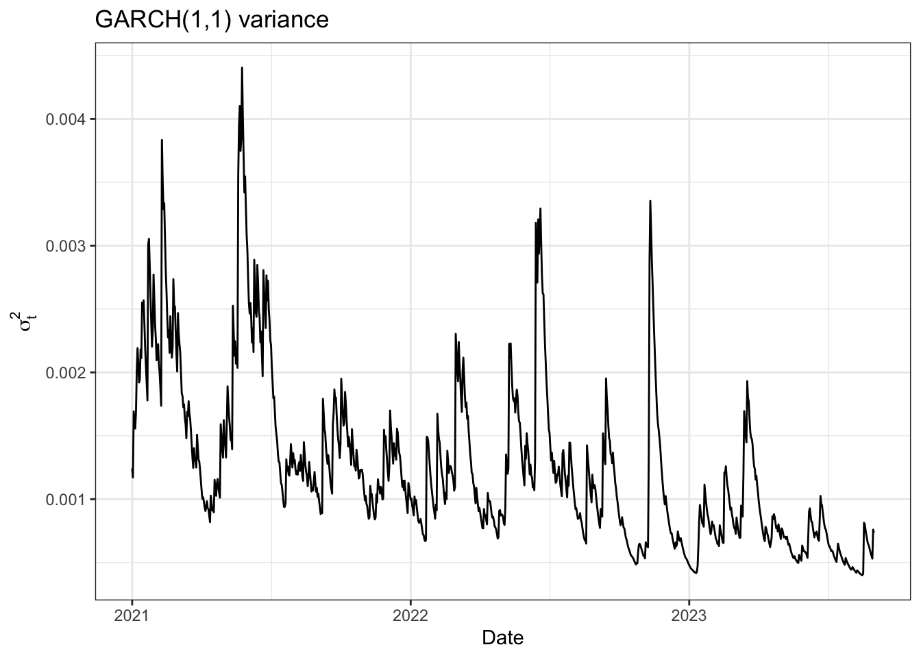
GARCH(1,1) variance

dplyr::tibble(t = df$date, sigma = fit@fit$var) %>%
  ggplot()+
  geom_line(aes(t, sigma)) +
  theme_bw()+
  labs(title = "GARCH(1,1) variance", y = TeX("$\\sigma_{t}^{2}$"), x = "Date")

4 Simulation of BTCUSD data

GARCH(1,1) simulations

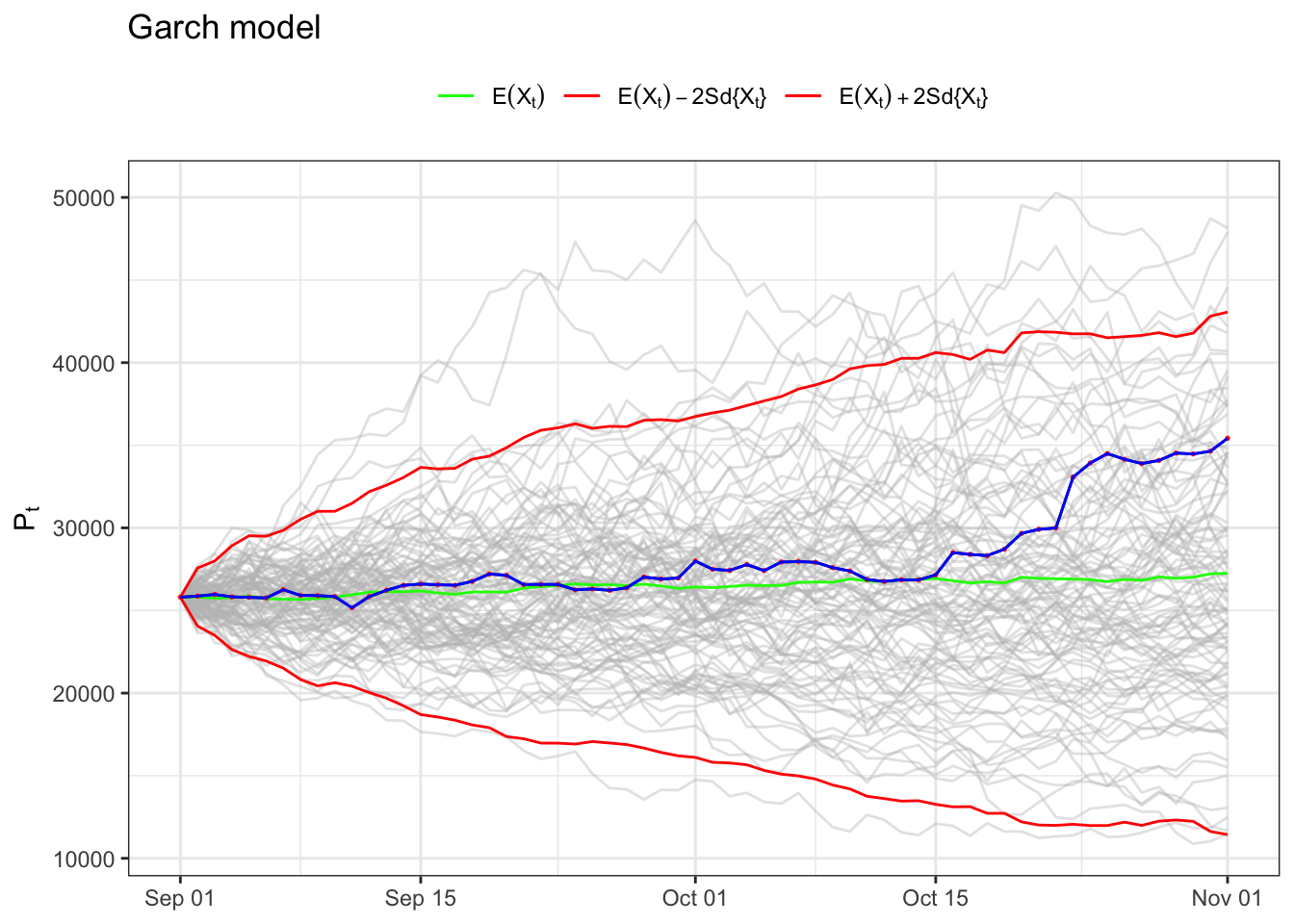
################### inputs ################### 
j_bar <- 100 # number of simulations 
seed <- 1
##############################################
set.seed(seed)

df_ <- dplyr::filter(df_fit, date >= as.Date(date_sim_from) & date <= as.Date(date_sim_to))
df_$t <- 1:nrow(df_)
S0 <- df_$Pt[1] # initial price 
nsim <- as.numeric(difftime(date_sim_to, date_sim_from))

# Garch model simulations
sim <- ugarchsim(fit, n.sim = nsim, m.sim = j_bar)
sim_ls <- list()
for(i in 1:j_bar){
  St <- sim@simulation$seriesSim[,i]
  Sigma <- c(sim@simulation$sigmaSim[,i][1], sim@simulation$sigmaSim[,i])
  sim_ls[[i]] <- dplyr::tibble(seed = i,
                               t = 1:(length(St)+1), 
                               St = c(0, St), 
                               Pt =  S0*cumprod(exp(St)),
                               Sigma = Sigma)
}
# dataset with simulations 
df_sim <- dplyr::bind_rows(sim_ls)
df_sim <- dplyr::left_join(df_sim, dplyr::select(df_, t, date), by = "t")

# dataset with mean path and standard deviations 
df2 <- df_sim %>%
  group_by(date) %>%
  summarise(EX = mean(Pt), Upper = EX + 2*sd(Pt), Lower = EX - 2*sd(Pt), 
            e_sigma = mean(Sigma), sigma_dw = mean(Sigma) + 2*sd(Sigma), sigma_up = mean(Sigma) - 2*sd(Sigma)) 

ggplot() +
  geom_line(data = df_sim, aes(date, Pt, group = seed), color = "gray", alpha = 0.4)+
  geom_line(data = df2, aes(date, EX, color = "expectation"))+
  geom_line(data = df2, aes(date, Upper, color = "upper"))+
  geom_line(data = df2, aes(date, Lower, color = "lower"))+
  geom_line(data = df_, aes(date, Pt), color = "black", alpha = 0.9)+
  geom_point(data = df_, aes(date, Pt), color = "red", alpha = 0.9, size = 0.3)+
  geom_line(data = df_, aes(date, Pt), color = "blue", alpha = 1)+
  scale_color_manual(values = c(upper = "red", lower = "red", expectation = "green"),
                     label = c(upper = latex2exp::TeX("$E(X_t) + 2Sd\\{X_t\\}$"),
                               lower = latex2exp::TeX("$E(X_t) - 2Sd\\{X_t\\}$"),
                               expectation = latex2exp::TeX("$E(X_t)$")))+
  labs(title = "Garch model", x = NULL, y = latex2exp::TeX("$P_t$"), color = "")+
  theme_bw()+
  theme(legend.position = "top")

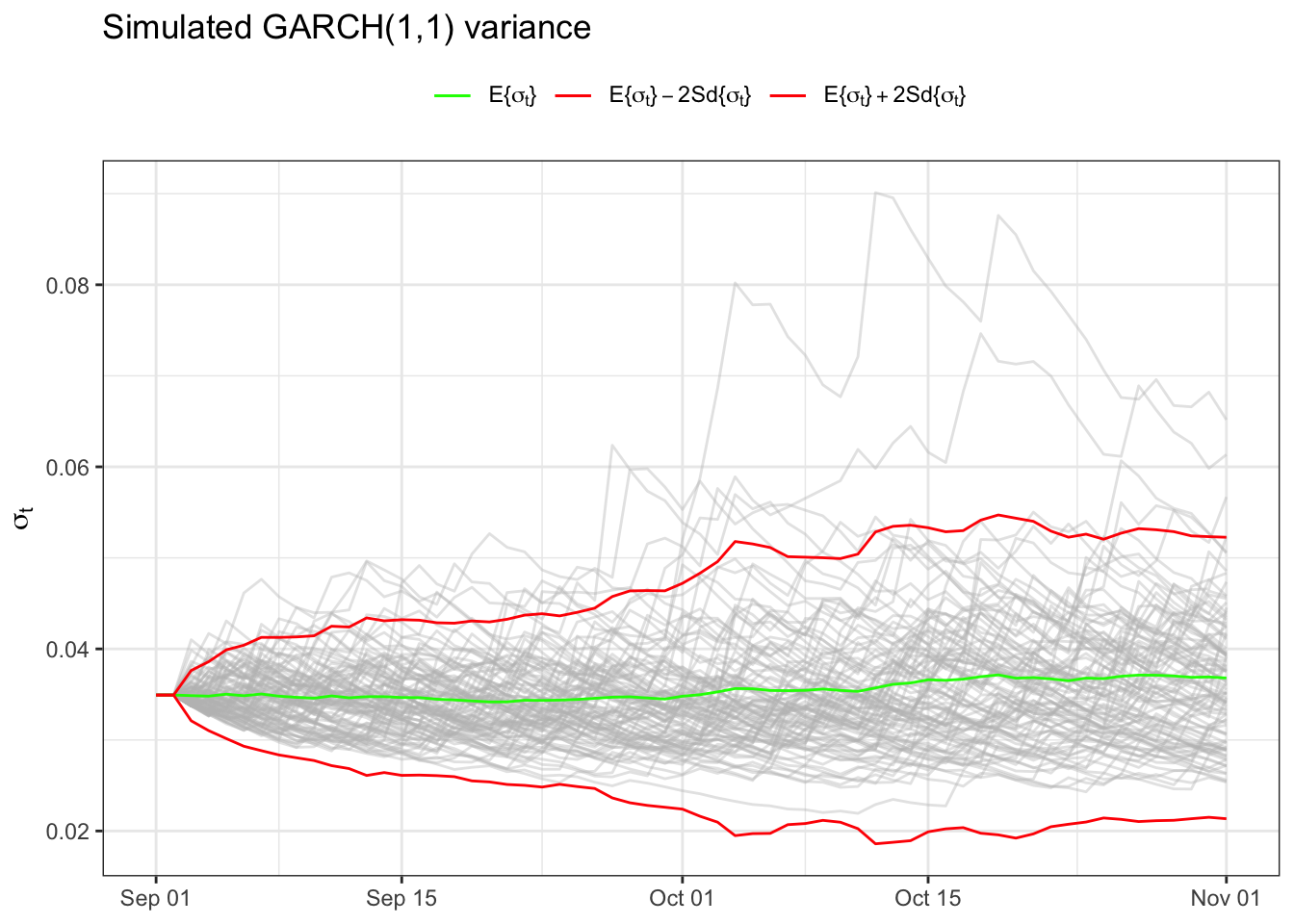
ggplot() +
  geom_line(data = df_sim[-1,], aes(date, Sigma, group = seed), color = "gray", alpha = 0.4)+
  geom_line(data = df2, aes(date, e_sigma, color = "expectation"))+
  geom_line(data = df2, aes(date, sigma_dw, color = "upper"))+
  geom_line(data = df2, aes(date, sigma_up, color = "lower"))+
  scale_color_manual(values = c(upper = "red", lower = "red", expectation = "green"),
                     label = c(upper = latex2exp::TeX("$E\\{\\sigma_t\\} + 2Sd\\{\\sigma_t\\}$"),
                               lower = latex2exp::TeX("$E\\{\\sigma_t\\} - 2Sd\\{\\sigma_t\\}$"),
                               expectation = latex2exp::TeX("$E\\{\\sigma_t\\}$")))+
  theme_bw()+
  theme(legend.position = "top") +
  labs(title = "Simulated GARCH(1,1) variance", y = TeX("$\\sigma_{t}$"), x = NULL, color = NULL)

Citation

BibTeX citation:

@online{sartini2023,
  author = {Sartini, Beniamino},
  title = {Modelling Approaches for {Bitcoin} Price},
  date = {2023-09-30},
  url = {https://cryptoverser.org/articles/garch-model-bitcoin/garch-model-bitcoin.html},
  langid = {en}
}

For attribution, please cite this work as:

Sartini, Beniamino. 2023. “Modelling Approaches for Bitcoin Price.” September 30, 2023. https://cryptoverser.org/articles/garch-model-bitcoin/garch-model-bitcoin.html.