Order Imbalance

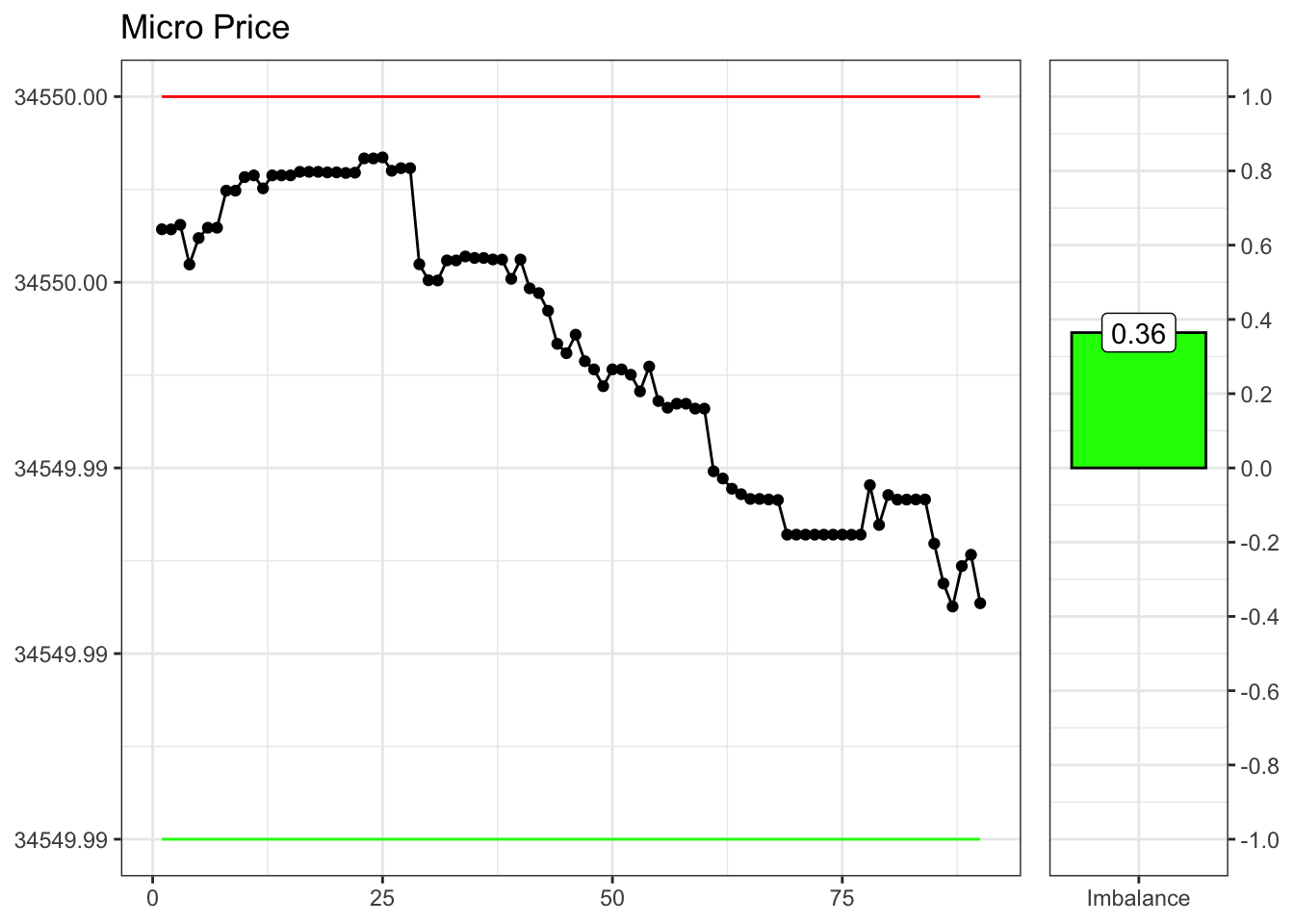
Following Lipton, Pesavento, and Sotiropoulos (2013) the order imbalance signal is defined as:

$$S_t^{imb}=\frac{q^{bid}-q^{ask}}{q^{bid}+q^{ask}}\in [-1,1]$$

Where

• $q^{bid}$ is the quantity at the Bid price.
• $q^{ask}$ is the quantity at the Ask price.

data <- head(df_ask_bid[-c(1:350),], n = 90)
# data <- group_by(data, date, pair) %>% summarise_all(mean)

data <- dplyr::mutate(data, 
                      t = c(1:nrow(data))[order(1:nrow(data), decreasing = TRUE)],
                      microprice = (bid*quantity_bid + ask*quantity_ask)/(quantity_bid + quantity_ask),
                      imbalance = (quantity_bid - quantity_ask)/(quantity_bid + quantity_ask),
                      label_imbalance = ifelse(imbalance > 0, "bid", "ask"))
plot_1 <-
ggplot(data) +
      geom_line(aes(t, microprice))+
      geom_point(aes(t, microprice))+
      geom_line(aes(t, ask), col = "red")+
      geom_line(aes(t, bid), col = "green")+
      theme_bw()+
      labs(
        title = "Micro Price",
        x = NULL, 
        y = NULL
      )
plot_2 <-
ggplot(data[1,]) +
      geom_bar(stat = "identity", aes("Imbalance", imbalance, fill = label_imbalance), col = "black")+
      geom_label(aes("Imbalance", imbalance, label = round(imbalance, 2)), col = "black")+
      scale_y_continuous(breaks = seq(-1, 1, 0.2), limits = c(-1, 1), position = "right")+
      scale_fill_manual(values = c(ask = "red", bid = "green"))+
      theme_bw()+
      labs(
        title = "",
        x = NULL, 
        y = NULL
      )+
  theme(legend.position = "none")

gridExtra::grid.arrange(plot_1, plot_2, ncol = 2, widths = c(80, 20))

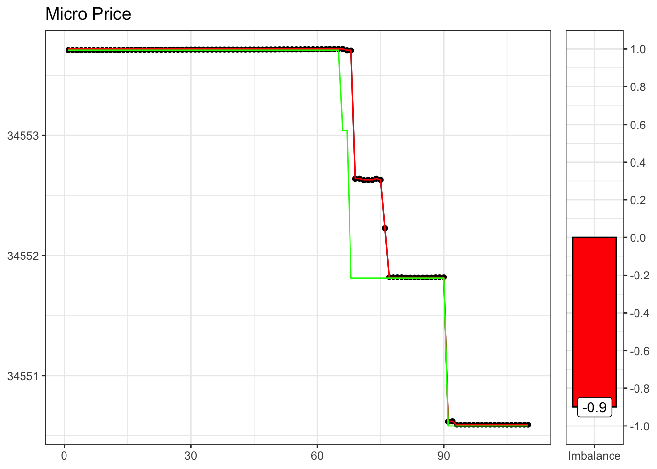
data <- head(df_ask_bid[-c(1:450),], n = 110)
# data <- group_by(data, date, pair) %>% summarise_all(mean)

data <- dplyr::mutate(data, 
                      t = c(1:nrow(data))[order(1:nrow(data), decreasing = TRUE)],
                      microprice = (bid*quantity_bid + ask*quantity_ask)/(quantity_bid + quantity_ask),
                      imbalance = (quantity_bid - quantity_ask)/(quantity_bid + quantity_ask),
                      label_imbalance = ifelse(imbalance > 0, "bid", "ask"))
plot_1 <-
ggplot(data) +
      geom_line(aes(t, microprice))+
      geom_point(aes(t, microprice))+
      geom_line(aes(t, ask), col = "red")+
      geom_line(aes(t, bid), col = "green")+
      theme_bw()+
      labs(
        title = "Micro Price",
        x = NULL, 
        y = NULL
      )
plot_2 <-
ggplot(data[1,]) +
      geom_bar(stat = "identity", aes("Imbalance", imbalance, fill = label_imbalance), col = "black")+
      geom_label(aes("Imbalance", imbalance, label = round(imbalance, 2)), col = "black")+
      scale_y_continuous(breaks = seq(-1, 1, 0.2), limits = c(-1, 1), position = "right")+
      scale_fill_manual(values = c(ask = "red", bid = "green"))+
      theme_bw()+
      labs(
        title = "",
        x = NULL, 
        y = NULL
      )+
  theme(legend.position = "none")

gridExtra::grid.arrange(plot_1, plot_2, ncol = 2, widths = c(85, 15))

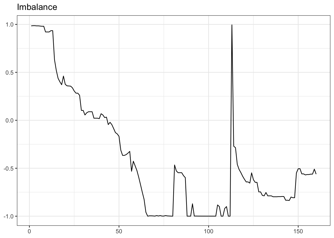
data <- head(df_ask_bid[-c(1:400),], n = 160)
# data <- group_by(data, date, pair) %>% summarise_all(mean)

data <- dplyr::mutate(data, 
                      t = c(1:nrow(data))[order(1:nrow(data), decreasing = TRUE)],
                      microprice = (bid*quantity_bid + ask*quantity_ask)/(quantity_bid + quantity_ask),
                      imbalance = (quantity_bid - quantity_ask)/(quantity_bid + quantity_ask),
                      label_imbalance = ifelse(imbalance > 0, "bid", "ask"))

ggplot(data) +
      geom_line(aes(t, imbalance))+
      theme_bw()+
      labs(
        title = "Imbalance",
        x = NULL, 
        y = NULL
      )

References

Lipton, Alexander, Umberto Pesavento, and Michael G Sotiropoulos. 2013. “Trade Arrival Dynamics and Quote Imbalance in a Limit Order Book.” https://arxiv.org/abs/1312.0514.

Citation

BibTeX citation:

@online{sartini2024,
  author = {Sartini, Beniamino},
  title = {Order {Imbalance}},
  date = {2024-01-17},
  url = {https://cryptoverser.org/articles/high-frequency/order-imbalance/order-imbalance.html},
  langid = {en}
}

For attribution, please cite this work as:

Sartini, Beniamino. 2024. “Order Imbalance.” January 17, 2024. https://cryptoverser.org/articles/high-frequency/order-imbalance/order-imbalance.html.