1 Order Book

An order book is a set of quantities and prices for a given time $t$ . Using a similar notation as in Gatheral and Oomen (2010), let’s define: - $p_{t, 1}^{b}$ : the best BID price at time $t$ . - $p_{t, 1}^{a}$ : the best ASK price at time $t$ . - $v_{t, 1}^{b}$ : quantity as limit buy order at the best BID price at time $t$ . - $v_{t, 1}^{a}$ : quantity as limit buy order at the best ASK price at time $t$ .

These quantities are usually ordered in such a way that: $v_{t, n_{a}}^{a} < v_{t, n_{a} - 1}^{a} < \dots < v_{t, 1}^{a} < v_{t, 1}^{b} < \dots < v_{t, n_{b} - 1}^{b} < v_{t, n_{b}}^{b}$ It follows that the prices will be ordered in a similar way: $p_{t, n_{a}}^{a} < p_{t, n_{a} - 1}^{a} < \dots < p_{t, 1}^{a} < p_{t, 1}^{b} < \dots < p_{t, n_{b} - 1}^{b} < p_{t, n_{b}}^{b}$

Quantity	Price
$v_{t, n_{a}}^{a}$	$p_{t, n_{a}}^{a}$
$v_{t, n_{a} - 1}^{a}$	$p_{t, n_{a} - 1}^{a}$
$⋮$	$⋮$
$v_{t, 2}^{a}$	$p_{t, 2}^{a}$
$v_{t, 1}^{a}$	$p_{t, 1}^{a}$
$v_{t, 1}^{b}$	$p_{t, 1}^{b}$
$v_{t, 2}^{b}$	$p_{t, 2}^{b}$
$⋮$	$⋮$
$v_{t, n_{b} - 1}^{b}$	$p_{t, n_{b} - 1}^{b}$
$v_{t, n_{b}}^{b}$	$p_{t, n_{b}}^{b}$

1.1 Mid-quote

The trade price and mid-quote series are commonly used in the literature. The micro-price, more familiar to practitioners, linearly weighs the bid and ask prices by the volume on the opposite side of the book and can thus be interpreted as the market clearing price when demand and supply curves are linear in price.

Show the code

# import depth data from binance 
library(binancer)
library(dplyr)
depth <- binance_depth(api = "spot", pair = "BTCUSDT", quiet = TRUE)

# best ask and bid 
bask <- tail(dplyr::filter(depth, side == "ASK"), n = 1) # best ask
bbid <- head(dplyr::filter(depth, side == "BID"), n = 1) # best bid

dplyr::bind_rows(bask, bbid) %>%
  knitr::kable() %>%
  kableExtra::kable_classic_2()

last_update_id	date	market	pair	side	price	quantity
47329760756	2024-05-24 14:33:31	spot	BTCUSDT	ASK	67430.01	6.51457
47329760756	2024-05-24 14:33:31	spot	BTCUSDT	BID	67430.00	1.51181

The mid-quote is computed as mean price among the best BID and ASK prices: $q_{t}^{m} = \frac{p_{t, 1}^{b} + p_{t, 1}^{a}}{2}$

Show the code

# compute mid-price 
bbid$mid_price  <- (bbid$price + bask$price)/2

bbid %>%
  dplyr::select(-side, -price, -quantity) %>%
  knitr::kable() %>%
  kableExtra::kable_classic_2()

last_update_id	date	market	pair	mid_price
47329760756	2024-05-24 14:33:31	spot	BTCUSDT	67430.01

1.2 BID-ASK Spread

The bid-ask spread is the mean distance between the best BID and ASK prices: $s_{t} = \frac{p_{t, 1}^{a} - p_{t, 1}^{b}}{2}$

Show the code

# compute bid-ask spread 
bbid$spread <- (bask$price - bbid$price)/2
bbid %>%
  dplyr::select(-side, -price, -quantity) %>%
  knitr::kable() %>%
  kableExtra::kable_classic_2()

last_update_id	date	market	pair	mid_price	spread
47329760756	2024-05-24 14:33:31	spot	BTCUSDT	67430.01	0.005

1.3 Micro Price

The micro-price $q_{t}^{v}$ is defined as weighted sum of the best BID-ASK by the quantities: $q_{t}^{v} = \frac{p_{t, 1}^{b} \cdot v_{t, 1}^{b} + p_{t, 1}^{a} \cdot v_{t, 1}^{a}}{v_{t, 1}^{b} + v_{t, 1}^{a}}$

Show the code

# compute micro-price 
bbid$micro_price <- (bbid$price*bbid$quantity + bask$price*bask$quantity)/(bbid$quantity + bask$quantity)

bbid %>%
  dplyr::select(-side, -price, -quantity) %>%
  knitr::kable() %>%
  kableExtra::kable_classic_2()

last_update_id	date	market	pair	mid_price	spread	micro_price
47329760756	2024-05-24 14:33:31	spot	BTCUSDT	67430.01	0.005	67430.01

2 Liquidity curve

Consider $n_{a} + n_{b}$ -levels in the order book. In order to compute the liquidity curve we arrange the quantities in ascending order: ${v_{t, n_{b}}^{b}, v_{t, n_{b} - 1}^{b}, \dots, v_{t, 1}^{b}, v_{t, 1}^{a}, \dots, v_{t, n_{a} - 1}^{a}, v_{t, n_{a}}^{a}}$ In order to build the liquidity curve we have to cumulate those quantities.

Show the code

library(ggplot2)
# order by price (descending)
plot_data <- dplyr::arrange(depth, price)
# Compute cumulated quantity 
plot_data$cum_quantity <- cumsum(plot_data$quantity)

ggplot()+
  geom_line(data = plot_data, aes(price, cum_quantity, color = side), size = 0.1)+
  geom_point(data = plot_data, aes(price, cum_quantity, color = side), size = 0.05)+
  scale_color_manual(values = c(ASK = "red", BID = "green"))+
  labs(x = "Price", 
       y = "Cumulated Quantity", 
       color = "Side", 
       caption = paste0("Last update: ", depth$date[1]))+
  theme(axis.title  = element_text(face = "bold"), 
        plot.title  = element_text(face = "bold"),
        axis.line = element_line(),
        axis.text.x = element_text(angle = 0, face = "bold", size = 7), 
        axis.text.y = element_text(face = "bold"), 
        axis.title.x = element_text(face = "bold",size = 10),
        axis.title.y = element_text(face = "bold", size = 10),
        plot.subtitle = element_text(face = "italic"),
        plot.caption = element_text(face = "italic"),
        panel.grid.minor.x = element_blank(),
        panel.grid.minor.y = element_blank(),
        panel.grid.major.x = element_blank(),
        panel.grid.major.y = element_blank(),
        panel.border = element_blank(),
        strip.background = element_blank(),
        panel.background = element_blank(),
        strip.text = element_text(angle = 0, face = "bold", size = 7), 
        legend.title = element_text(face = "bold", size = 11),
        legend.text = element_text(face = "italic", size = 10),
        legend.box.background = element_rect(),
        legend.position = "none")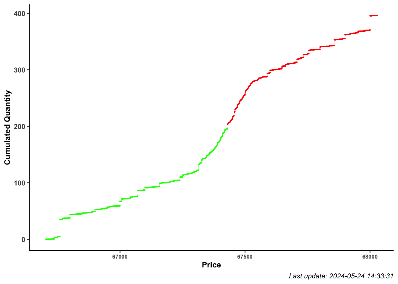

Show the code

library(ggplot2)
depth_level <- 0.0001 # i.e. 0.01 %
# Arrange the prices in descending order
plot_data <- dplyr::arrange(depth, price)
# Compute cumulated quantity 
plot_data$cum_quantity <- cumsum(plot_data$quantity)
# Index best ASK and BID 
idx_best_ASK <- which(plot_data$side == "ASK")[1]
idx_best_BID <- idx_best_ASK - 1
# Microprice coordinates 
x <- bbid$price
y <- plot_data$cum_quantity[idx_best_BID]
xend <- bask$price
yend <- plot_data$cum_quantity[idx_best_ASK]
mp <- c(x, xend, y, yend)
# Zoom dataset 
plot_data <- filter(plot_data, price >= bbid$micro_price*(1 - depth_level) & price <= bbid$micro_price*(1 + depth_level))

ggplot()+
  geom_line(data = plot_data, aes(price, cum_quantity, color = side), size = 0.4)+
  geom_point(data = plot_data, aes(price, cum_quantity), color = "black", size = 0.8)+
  geom_point(data = plot_data, aes(price, cum_quantity, color = side), size = 0.4)+
  geom_segment(aes(x = mp[1], xend = mp[2], y = mp[3], yend = mp[4]), linetype="dashed", color = "red")+
  geom_point(aes(x = mp[1], y = mp[4]), size=1.3, color = "black")+
  geom_point(aes(x = mp[1], y = mp[4]), size=0.9, color = "red")+
  geom_point(aes(x = mp[2], y = mp[3]), size=1.3, color = "black")+
  geom_point(aes(x = mp[2], y = mp[3]), size=0.9, color = "green")+
  scale_color_manual(values = c(ASK = "red", BID = "green"))+
  labs(x = "Price", 
       y = "Cumulated Quantity", 
       color = "Side", 
       caption = paste0("Last update: ", depth$date[1]))+
  theme(axis.title  = element_text(face = "bold"), 
        plot.title  = element_text(face = "bold"),
        axis.line = element_line(),
        axis.text.x = element_text(angle = 0, face = "bold", size = 7), 
        axis.text.y = element_text(face = "bold"), 
        axis.title.x = element_text(face = "bold",size = 10),
        axis.title.y = element_text(face = "bold", size = 10),
        plot.subtitle = element_text(face = "italic"),
        plot.caption = element_text(face = "italic"),
        panel.grid.minor.x = element_blank(),
        panel.grid.minor.y = element_blank(),
        panel.grid.major.x = element_blank(),
        panel.grid.major.y = element_blank(),
        panel.border = element_blank(),
        strip.background = element_blank(),
        panel.background = element_blank(),
        strip.text = element_text(angle = 0, face = "bold", size = 7), 
        legend.title = element_text(face = "bold", size = 11),
        legend.text = element_text(face = "italic", size = 10),
        legend.box.background = element_rect(),
        legend.position = "none")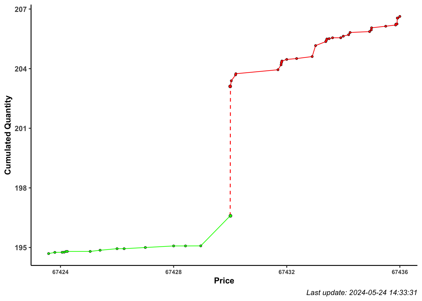

2.1 Depth curve

Show the code

# ASK orders 
ask <- dplyr::filter(depth, side == "ASK") 
# Arrange by price (descending) 
ask <- dplyr::arrange(ask, price)
# Compute cumulated quantity 
ask$cum_quantity <- cumsum(ask$quantity)
# BID orders 
bid <- dplyr::filter(depth, side == "BID")
# Arrange by price (ascending) 
bid <- dplyr::arrange(bid, dplyr::desc(price))
# Compute cumulated quantity 
bid$cum_quantity <- cumsum(bid$quantity) 

x_breaks <- c(seq(min(bid$price), bbid$micro_price, length.out = 3), seq(bbid$micro_price, max(ask$price), length.out = 3))

ggplot()+
  geom_line(data = dplyr::bind_rows(ask, bid), aes(price, cum_quantity, color = side))+
  geom_point(aes(bbid$micro_price, 0), color = "black")+
  scale_color_manual(values = c(ASK = "red", BID = "green"))+
  scale_x_continuous(breaks = x_breaks, labels = round(x_breaks, 2))+
  labs(x = "Price", 
       y = "Quantity", 
       color = "Side", 
       caption = paste0("Last update: ", depth$date[1]))+
  theme(axis.title  = element_text(face = "bold"), 
        plot.title  = element_text(face = "bold"),
        axis.line = element_line(),
        axis.text.x = element_text(angle = 0, face = "bold", size = 7), 
        axis.text.y = element_text(face = "bold"), 
        axis.title.x = element_text(face = "bold",size = 10),
        axis.title.y = element_text(face = "bold", size = 10),
        plot.subtitle = element_text(face = "italic"),
        plot.caption = element_text(face = "italic"),
        panel.grid.minor.x = element_blank(),
        panel.grid.minor.y = element_blank(),
        panel.grid.major.x = element_blank(),
        panel.grid.major.y = element_blank(),
        panel.border = element_blank(),
        strip.background = element_blank(),
        panel.background = element_blank(),
        strip.text = element_text(angle = 0, face = "bold", size = 7), 
        legend.title = element_text(face = "bold", size = 11),
        legend.text = element_text(face = "italic", size = 10),
        legend.box.background = element_rect(),
        legend.position = "none")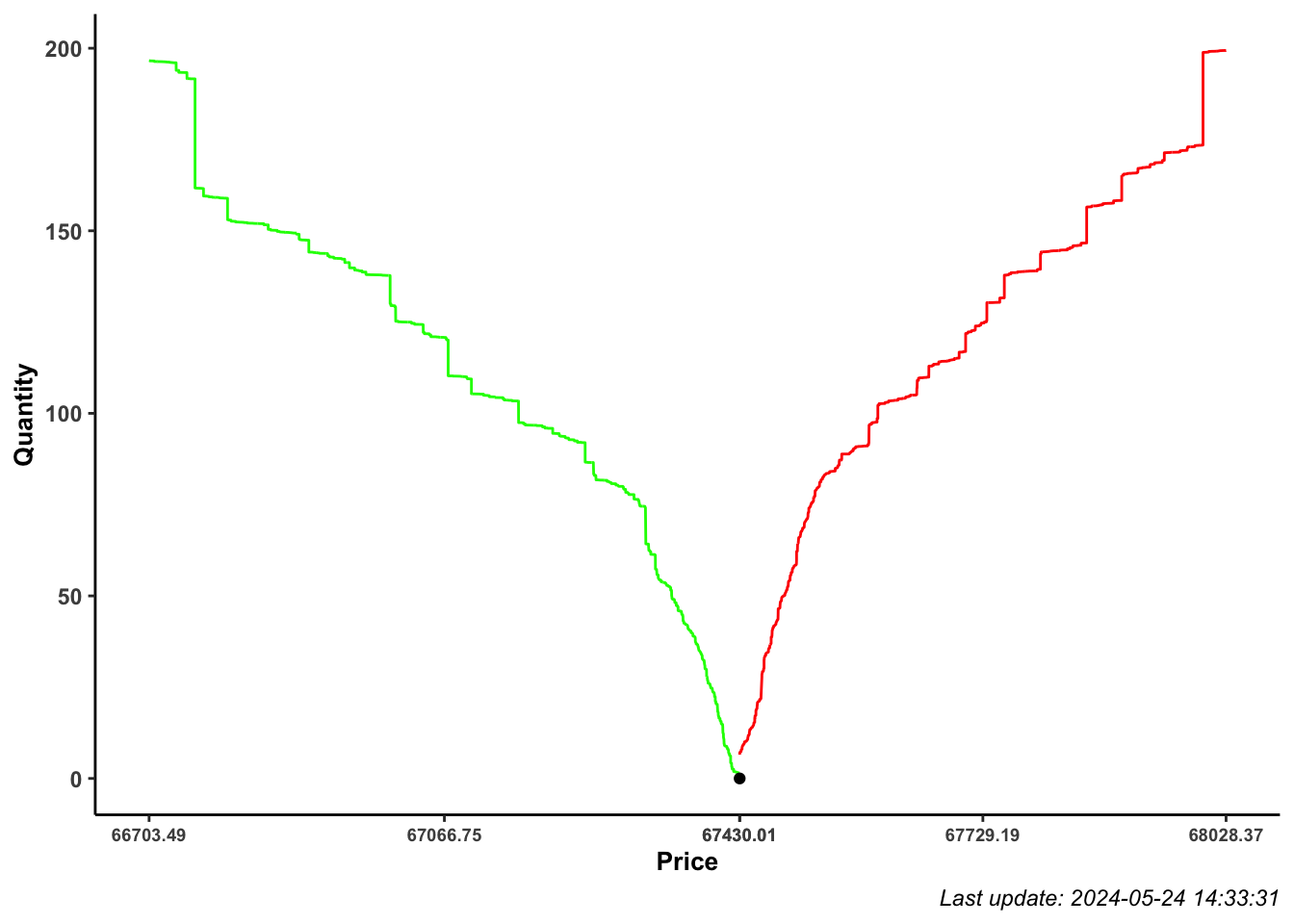

References

Gatheral, Jim, and Roel Oomen. 2010. “Zero-Intelligence Realized Variance Estimation.” Finance and Stochastics. https://papers.ssrn.com/sol3/papers.cfm?abstract_id=970358.

Citation

BibTeX citation:

@online{sartini2024,
  author = {Sartini, Beniamino},
  title = {Microprice and {Liquidity} {Curve}},
  date = {2024-01-17},
  url = {https://cryptoverser.org/articles/signals-microprice/signals-microprice.html},
  langid = {en}
}

For attribution, please cite this work as:

Sartini, Beniamino. 2024. “Microprice and Liquidity Curve.” January 17, 2024. https://cryptoverser.org/articles/signals-microprice/signals-microprice.html.