Simple rebalance strategy

Trading
Author

Beniamino Sartini

Published

October 18, 2023

1 Rebalance Strategy

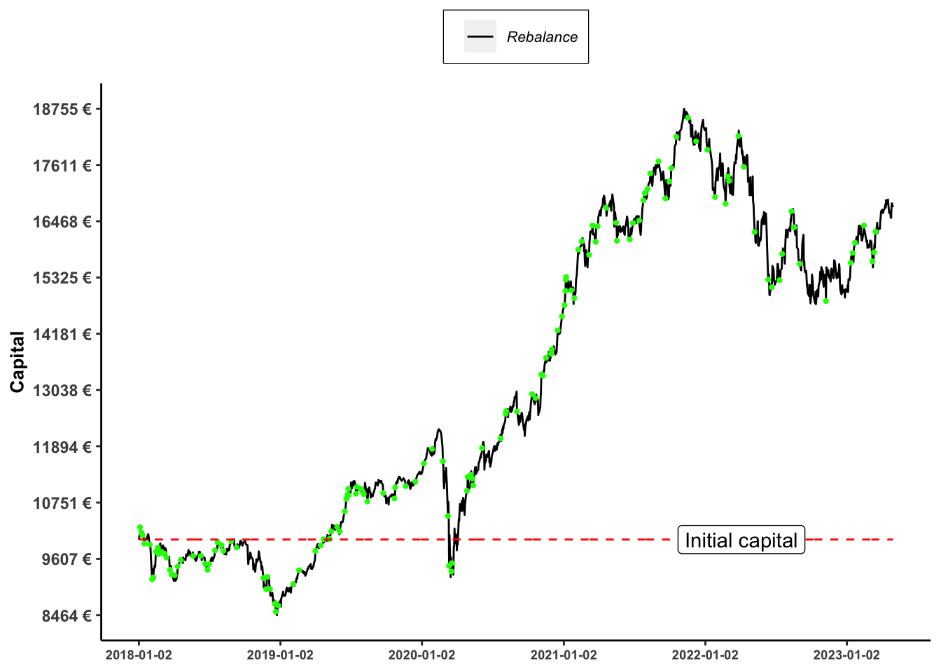
A re-balance strategy consists in a portfolio \(\Pi\), with \(\bar{n}\)-assets whose relative weights \(w\) need to be constant and equal to an ideal allocation \(w^{\star}\). Let’s consider the following situation:

  • the portfolio \(\Pi\) is self-financing: a capital is invested at time \(t_{now}\) and the profit and losses (\(P\&L\)) are generated by the returns of the instruments inside the portfolio.

  • The assets available are in dollars, but the investment capital is expressed in euros (€). In this way we simulate the situation of an European investor that have to deal with the currency risk coming from the fact that the assets are not quoted in the domestic currency (euros).

  • We consider also the transaction costs, but not (eventual) capital gain taxes. Moreover, in order to avoid to re-balance too often, we set an additional parameter \(\epsilon \in [0,1)\) to contro it. In this way the rebalance will occur only if the weight of an asset, i.e. \(w\), exceed the following bounds with respect to the ideal weight \(w^{\star}\): \[w^{\star} (1-\epsilon ) \leq w \leq w^{\star} (1+\epsilon) \; \; \Rightarrow \; \; \text{no rebalance}\]

1.1 Implementation in R

Show the inputs
require("dplyr")   # for data manipulation 
require("ggplot2") # for plots 
require("readr")   # for importing data (or simply read.csv)

# risky assets 
dataset <- readr::read_csv("dataset.csv", show_col_types = FALSE)
# initial date for the strategy
t_now <- as.Date("2018-01-01")
# end date for the strategy
t_hor <- as.Date("2023-05-01") 
# capital invested at time t_now 
initial_capital <- 10000
# ideal weights of risky assets
w_risky = c(BTC = 0.1, SP500 = 0.6, GOLD = 0.1, USDEUR = 0.2)
# implied risk-free investments (liquid cash in EUR)
w_riskfree = max(1 - sum(w_risky), 0)
# tolerance  to avoid a re-balancing a small quantity 
w_tolerance = 0.10
# Transaction fee 
tx_fee <- 0.1/100

# filter risk_asset dataset to be in [t_now, t_hor] 
dataset <- dataset[dataset$date >= t_now & dataset$date <= t_hor,]
# select the assets 
risky_asset <- dataset[,colnames(dataset) %in% c("date", names(w_risky))]
# update t_now with the most recent date if t_now is an holiday
t_now <- min(risky_asset$date)
# select the prices at time t_now 
price_now <- unlist(risky_asset[risky_asset$date == t_now,][,-1])

We consider a capital of 10000€ invested in 2018-01-02 up to 2023-05-01. We consider a portfolio composed by Bitcoin (10%), the S&P500 index (60%), Gold spot (10%) and the remaining part liquid in USD (20%). The rebalances will occur in the following bounds:

Asset \(w^{\star} (1-\epsilon )\) \(w^{\star}\) \(w^{\star} (1+\epsilon )\) Value
BITCOIN 9% 10% 11% 1000€
S&P500 54% 60% 66% 6000€
GOLD 9% 10% 11% 1000€
USD 18% 20% 22% 2000€
Show the initialization
# initialize risky investments dataset 
df_risky <- dplyr::tibble( date = t_now, 
                           # risky asset symbols 
                           symbol = colnames(risky_asset)[-1],  
                           # risky asset prices at t_now 
                           price = price_now,
                           # risky asset weights 
                           weights = w_risky,
                           # risky asset total value at t_now 
                           value = initial_capital*weights,
                           # risky asset holdings amount at t_now 
                           holdings = value/price )

# initialize risk-free investments dataset
df_riskfree <- dplyr::tibble(date = t_now, 
                             # risky asset symbols 
                             symbol = "EUR",  
                             # riskfree asset prices at t_now 
                             price = 1,
                             # risky asset weights 
                             weights = w_riskfree,
                             # risky asset total value at t_now 
                             value =  initial_capital*weights,
                             # risky asset holdings amount at t_now 
                             holdings = value/price )

# initialize the portfolio
df_portfolio <- dplyr::tibble(date = t_now, # time now 
                              symbol = "Portfolio",  
                              capital = initial_capital, # initial capital
                              rebalance = FALSE, # if TRUE has happened a rebalance 
                              change = 0) # return 
Show the re-balance
fees <- 0
# initialize a list to store each rebalance 
strategy <- list()
strategy[[1]] <- list()
strategy[[1]]$risky <- df_risky
strategy[[1]]$riskfree <- df_riskfree
strategy[[1]]$portfolio <- df_portfolio
for(i in 2:nrow(risky_asset)){
  # start from the previous rebalance
  strat <- strategy[[i-1]] 
  # update the date in all the lists 
  strat$risky$date <- risky_asset$date[i]
  strat$riskfree$date <- risky_asset$date[i]
  strat$portfolio$date <- risky_asset$date[i]
  # update prices for risky assets 
  strat$risky$price <- unlist(risky_asset[i,][,-1])
  # Update weights and portfolio value 
  # compute value of risky assets given holdings at previous time 
  strat$risky$value <- strat$risky$holdings*strat$risky$price
  # update value of total capital 
  strat$portfolio$capital <- strat$riskfree$value + sum(strat$risky$value)
  # compute actual weights of risky assets
  strat$risky$weights <- strat$risky$value/strat$portfolio$capital
  # compute target value of risky assets given ideal allocation 
  target_risky_value <- strat$portfolio$capital*w_risky
  # Re-balance 
  # h_reb positive imply BUY while h_reb negative imply SELL
  h_reb <- (target_risky_value - strat$risky$value)/strat$risky$price
  # check tolerance bounds: re-balance only if weights exceed bounds
  w_actual <- strat$risky$weights
  w_star_up <- w_risky*(1 + w_tolerance)
  w_star_dw <- w_risky*(1 - w_tolerance)
  index_tolerance <- w_actual <= w_star_dw | w_actual >= w_star_up
  # set to zero the quantity for non-rebalancing assets 
  h_reb[!index_tolerance] = 0
  # check if no rebalances occurs 
  if(sum(index_tolerance != 0)){
    # add TRUE if re-belance happens 
    strat$portfolio$rebalance <- TRUE
  } else {
    # add FALSE if re-belance does not happen
    strat$portfolio$rebalance <- FALSE
  }
  # update holdings 
  strat$risky$holdings <- strat$risky$holdings + h_reb
  fees <- abs(h_reb*strat$risky$price*tx_fee)
  # update value of the risky assets given new weights 
  strat$risky$value <- strat$risky$holdings*strat$risky$price - fees
  # update capital in EUR h_reb positive means buy so we have sign reverted
  strat$riskfree$value <- strat$riskfree$value - sum(h_reb*strat$risky$price)
  # update portfolio value
  strat$portfolio$capital <- sum(strat$risky$value) + strat$riskfree$value
  # check that new weights are equal to ideal allocation 
  strat$risky$weights <- strat$risky$value/strat$portfolio$capital
  # drow-down: compute portfolio percentage change with respect to initial capital
  strat$portfolio$change <- (strat$portfolio$capital - initial_capital)/initial_capital
  # add to strategy list 
  strategy[[i]] <- strat
}
# data-set with the re-balancing strategy 
portfolio <- purrr::map_df(strategy, ~.x$portfolio)

2 Evaluation

Show the code
# scale x-axes 
x_levels <- seq.Date(min(as.Date(portfolio$date)), max(as.Date(portfolio$date)), by = "1 year")
# scale y-axes 
min_y <- min(portfolio$capital)
max_y <- max(portfolio$capital)
y_levels <- round(seq(min_y, max_y, length.out = 10))

plot_portfolio <- ggplot() +
  geom_line(data = portfolio, aes(date, capital, color = "reb_strat"))+
  geom_point(data = portfolio[portfolio$rebalance,], aes(date, capital), color = "green", size = 0.8) +
  geom_line(data = portfolio, aes(date, initial_capital), linewidth = 0.5, color = "red", linetype = "dashed") + 
  geom_label(data = portfolio[trunc(nrow(portfolio)/5*4),], aes(date, initial_capital, label = "Initial capital"))+
  labs(x = NULL, y = "Capital", color = NULL) +
  scale_color_manual(values = c(reb = "green", reb_strat = "black", 
                               bh_gold = "violet", bh_sp500 = "blue", bh_sp500_btc = "orange"), 
                     labels = c(reb = "R", reb_strat = "Rebalance", 
                                bh_gold = "Buy&Hold (Gold)", bh_sp500 = "Buy&Hold (S&P500)", 
                                bh_sp500_btc = "Buy&Hold (S&P500 + BTC)")) + 
  scale_y_continuous(labels = paste0(y_levels, " €"), breaks = y_levels) + 
  scale_x_date(breaks = x_levels)+
  ggtheme

plot_portfolio

2.1 Rebalance vs Buy&Hold S&P 500

Show the code
# buy and hold: SP500 
portfolio$bh_sp500 <- initial_capital/dataset$SP500[1]*dataset$SP500
# scale y-axes 
min_y <- min(portfolio$capital, portfolio$bh_sp500)
max_y <- max(portfolio$capital, portfolio$bh_sp500)
y_levels <- round(seq(min_y, max_y, length.out = 10))
# plot
plot_portfolio <- plot_portfolio + 
  geom_line(data = portfolio, aes(date, bh_sp500, color = "bh_sp500"), alpha = 0.5) +
  scale_y_continuous(labels = paste0(y_levels, " €"), breaks = y_levels)
plot_portfolio

2.2 Rebalance vs Buy&Hold Gold

Show the code
# buy and hold: Gold 
portfolio$bh_gold <- initial_capital/dataset$GOLD[1]*dataset$GOLD
# scale y-axes 
min_y <- min(portfolio$capital, portfolio$bh_sp500, portfolio$bh_gold)
max_y <- max(portfolio$capital, portfolio$bh_sp500, portfolio$bh_gold)
y_levels <- round(seq(min_y, max_y, length.out = 10))
# plot
plot_portfolio <- plot_portfolio + 
  geom_line(data = portfolio, aes(date, bh_gold, color = "bh_gold"), alpha = 0.5) +
  scale_y_continuous(labels = paste0(y_levels, " €"), breaks = y_levels)
plot_portfolio

2.3 Rebalance vs Buy&Hold S&P 500 and BTC

Show the code
# buy and hold: 50% Bitcoin and 50% Sp500
bh_btc <- 0.5*initial_capital/dataset$BTC[1]*dataset$BTC
bh_sp500 <- 0.5*initial_capital/dataset$SP500[1]*dataset$SP500
portfolio$bh_btc_sp500 <- bh_btc + bh_sp500
# scale y-axes 
min_y <- min(portfolio$capital, portfolio$bh_sp500, portfolio$bh_gold, portfolio$bh_btc_sp500)
max_y <- max(portfolio$capital, portfolio$bh_sp500, portfolio$bh_gold, portfolio$bh_btc_sp500)
y_levels <- round(seq(min_y, max_y, length.out = 10))
# plot 
plot_portfolio <- plot_portfolio + 
  geom_line(data = portfolio, aes(date, bh_btc_sp500, color = "bh_sp500_btc"), alpha = 0.5) +
  scale_y_continuous(labels = paste0(y_levels, " €"), breaks = y_levels) 
plot_portfolio

3 Conclusions

Show the code
# function to summarise a porfolio 
summarise_portfolio <- function(x, label = "portfolio"){
  
  # length of x ~ number of observations
  nobs <- length(x)
  # returns x should be a price not a return
  ret <- (x - dplyr::lag(x))/dplyr::lag(x)
  # daily mean (in percentage) 
  mu_ret <- mean(ret[-1], na.omit = TRUE)*100
  # daily standard deviation (in percentage) 
  sigma_ret <- sd(ret[-1])*100
  # max return (in percentage) 
  max_ret <- max((x - x[1])/x[1])*100
  # max drowdown (in percentage) 
  max_dd <- min((x - x[1])/x[1])*100
  # actual return 
  ret_t_now <- (x[nobs] - x[1])/x[1]*100
  # annualized return 
  ret_annual <- ret_t_now/(nobs/365)
  
  df <- dplyr::tibble(
    portfolio = label, 
    daily_stdev = sigma_ret, 
    max_dd = max_dd, 
    tot_ret = ret_t_now, 
    yearly_ret = ret_annual,
  )
}

dplyr::bind_rows(
  summarise_portfolio(portfolio$capital, label = "rebalance"),
  summarise_portfolio(portfolio$bh_sp500, label = "b&h Sp500"),
  summarise_portfolio(portfolio$bh_gold, label = "b&h Gold"),
  summarise_portfolio(portfolio$bh_btc_sp500, label = "b&h Btc + Sp500"),
) %>%
  dplyr::mutate_if(is.numeric, function(x) x/100) %>%
  mutate(initial = initial_capital, actual = initial_capital*(1+tot_ret)) %>%
  DT::datatable(filter = "none", options = list(dom = 't',
  initComplete = DT::JS(
    "function(settings, json) {",
    "$(this.api().table().header()).css({'background-color': '#000', 'color': '#fff'});",
    "}"))) %>%
  DT::formatCurrency(c("initial", "actual"), currency = "€", digits = 0, mark = "") %>%
  DT::formatPercentage(c("daily_stdev", "max_dd", "tot_ret", "yearly_ret"), digits = 2) 
Back to top

Citation

BibTeX citation:
@online{sartini2023,
  author = {Sartini, Beniamino},
  title = {Simple Rebalance Strategy},
  date = {2023-10-18},
  url = {https://cryptoverser.org/articles/trading-rebalance-strategy/rebalance_strategy.html},
  langid = {en}
}
For attribution, please cite this work as:
Sartini, Beniamino. 2023. “Simple Rebalance Strategy.” October 18, 2023. https://cryptoverser.org/articles/trading-rebalance-strategy/rebalance_strategy.html.